
经过数据预处理和特征选择,我们已经成功生成了一组优质的特征子集。然而,这组子集可能仍然包含过多的特征,导致训练模型时需要消耗过多的计算资源。在这种情况下,我们可以运用降维技术进一步压缩特征子集,但这可能会影响模型的性能。
与此同时,如果时间有限,我们也可以在数据预处理后直接采用降维方法,将原始特征空间压缩成新的特征子集。
在本文中,我们将详细介绍两种常用的降维技术:PCA(主成分分析)和LDA(线性判别分析)。
项目地址:
https://www.php.cn/link/e75b50aaf9e8125e58481a0cff44b539
本文将探讨特征工程中的特征降维技术。
目录:
1.1 非监督方法
1.1.1 主成分分析(PCA)
主成分分析(PCA)是一种无监督的机器学习技术,其目的是通过线性变换将原始特征投影到一系列线性无关的单位向量上,同时尽可能保留原始数据的信息(方差)。更多数学细节可在我们Github上的repo中查看。
https://www.php.cn/link/36f3776e5d1d89eed81547772a9d6a4f
代码语言:javascript代码运行次数:0运行复制```javascript import numpy as np import pandas as pd from sklearn.decomposition import PCA
from sklearn.datasets import fetch_california_housing dataset = fetch_california_housing() X, y = dataset.data, dataset.target # 使用 california_housing 数据集来演示
train_set = X[0:15000,:] test_set = X[15000:,] train_y = y[0:15000]
from sklearn.preprocessing import StandardScaler model = StandardScaler() model.fit(train_set) standardized_train = model.transform(train_set) standardized_test = model.transform(test_set)
compressor = PCA(n_components=0.9) # 将n_components设置为0.9 =>
compressor.fit(standardized_train) # 在训练集上训练 transformed_trainset = compressor.transform(standardized_train) # 转换训练集 (20000,5)
transformed_testset = compressor.transform(standardized_test) # 转换测试集 assert transformed_trainset.shape[1] == transformed_testset.shape[1] # 转换后训练集和测试集有相同的特征数
代码语言:javascript代码运行次数:0<svg fill="none" height="16" viewbox="0 0 16 16" width="16" xmlns="http://www.w3.org/2000/svg"><path d="M6.66666 10.9999L10.6667 7.99992L6.66666 4.99992V10.9999ZM7.99999 1.33325C4.31999 1.33325 1.33333 4.31992 1.33333 7.99992C1.33333 11.6799 4.31999 14.6666 7.99999 14.6666C11.68 14.6666 14.6667 11.6799 14.6667 7.99992C14.6667 4.31992 11.68 1.33325 7.99999 1.33325ZM7.99999 13.3333C5.05999 13.3333 2.66666 10.9399 2.66666 7.99992C2.66666 5.05992 5.05999 2.66659 7.99999 2.66659C10.94 2.66659 13.3333 5.05992 13.3333 7.99992C13.3333 10.9399 10.94 13.3333 7.99999 13.3333Z" fill="currentcolor"></path></svg>运行<svg fill="none" height="16" viewbox="0 0 16 16" width="16" xmlns="http://www.w3.org/2000/svg"><path clip-rule="evenodd" d="M4.5 15.5V3.5H14.5V15.5H4.5ZM12.5 5.5H6.5V13.5H12.5V5.5ZM9.5 2.5H3.5V12.5H1.5V0.5H11.5V2.5H9.5Z" fill="currentcolor" fill-rule="evenodd"></path></svg>复制```javascript
# 可视化 所解释的方差与选取的主成分数目之间的关系
import matplotlib.pyplot as plt
plt.rcParams['font.sans-serif']=['SimHei']
%matplotlib inline
plt.plot(np.array(range(len(compressor.explained_variance_ratio_))) + 1,
         np.cumsum(compressor.explained_variance_ratio_))
plt.xlabel('选取的主成分数目')
plt.ylabel('累计所解释的方差累')
plt.show(); # 前5个主成分可以保证保留原特征中90%的方差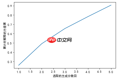
1.2 监督方法
1.2.1 线性判别分析(LDA)
与PCA不同,线性判别分析(LDA)是一种有监督的机器学习技术,其目标是找到一个特征子集,使得类别之间的线性可分性最大化,即希望同一类别数据的投影点尽可能接近,而不同类别数据的类别中心之间的距离尽可能大。LDA主要用于分类问题,并假设各类别的样本数据符合高斯分布且具有相同的协方差矩阵。
更多关于LDA原理的详细信息可以在sklearn的官方网站上找到。LDA会将原始变量压缩为(K-1)个,其中K是目标变量的类别数。但在sklearn中,通过将PCA的思想整合到LDA中,可以进一步压缩变量。
代码语言:javascript代码运行次数:0运行复制```javascript import numpy as np import pandas as pd from sklearn.discriminant_analysis import LinearDiscriminantAnalysis as LDA
from sklearn.datasets import load_iris iris = load_iris() X, y = iris.data, iris.target
np.random.seed(1234) idx = np.random.permutation(len(X)) X = X[idx] y = y[idx]
train_set = X[0:100,:] test_set = X[100:,] train_y = y[0:100] test_y = y[100:,]
from sklearn.preprocessing import StandardScaler # 我们也可以采用幂次变换 model = StandardScaler() model.fit(train_set) standardized_train = model.transform(train_set) standardized_test = model.transform(test_set)
compressor = LDA(n_components=2) # 将n_components设置为2
代码语言:javascript代码运行次数:0<svg fill="none" height="16" viewbox="0 0 16 16" width="16" xmlns="http://www.w3.org/2000/svg"><path d="M6.66666 10.9999L10.6667 7.99992L6.66666 4.99992V10.9999ZM7.99999 1.33325C4.31999 1.33325 1.33333 4.31992 1.33333 7.99992C1.33333 11.6799 4.31999 14.6666 7.99999 14.6666C11.68 14.6666 14.6667 11.6799 14.6667 7.99992C14.6667 4.31992 11.68 1.33325 7.99999 1.33325ZM7.99999 13.3333C5.05999 13.3333 2.66666 10.9399 2.66666 7.99992C2.66666 5.05992 5.05999 2.66659 7.99999 2.66659C10.94 2.66659 13.3333 5.05992 13.3333 7.99992C13.3333 10.9399 10.94 13.3333 7.99999 13.3333Z" fill="currentcolor"></path></svg>运行<svg fill="none" height="16" viewbox="0 0 16 16" width="16" xmlns="http://www.w3.org/2000/svg"><path clip-rule="evenodd" d="M4.5 15.5V3.5H14.5V15.5H4.5ZM12.5 5.5H6.5V13.5H12.5V5.5ZM9.5 2.5H3.5V12.5H1.5V0.5H11.5V2.5H9.5Z" fill="currentcolor" fill-rule="evenodd"></path></svg>复制```javascript
# 可视化 所解释的方差与选取的特征数目之间的关系
import matplotlib.pyplot as plt
plt.plot(np.array(range(len(compressor.explained_variance_ratio_))) + 1,
         np.cumsum(compressor.explained_variance_ratio_))
plt.xlabel('选取的特征数目')
plt.ylabel('累计所解释的方差累')
plt.show(); # LDA将原始的4个变量压缩为2个,这2个变量即能解释100%的方差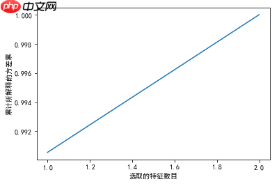
中文版 Jupyter 地址:
https://www.php.cn/link/3aed873670ec4df5ec69019f310a2d19
以上就是【完结篇】专栏 | 基于 Jupyter 的特征工程手册:特征降维的详细内容,更多请关注php中文网其它相关文章!

每个人都需要一台速度更快、更稳定的 PC。随着时间的推移,垃圾文件、旧注册表数据和不必要的后台进程会占用资源并降低性能。幸运的是,许多工具可以让 Windows 保持平稳运行。

 广告
广告Copyright 2014-2025 https://www.php.cn/ All Rights Reserved | php.cn | 湘ICP备2023035733号


 100
100