一文搞懂卷积网络之四（空间注意力Non-local）-人工智能-PHP中文网

本文介绍CNN注意力机制开篇之作Non-local，其解决传统CNN长距离特征提取不足问题，通过学习特征图点间相关性实现全局联系。文中实现了Embedded Gaussian等三种模块结构，在Cifar10上与ResNet18基线对比实验，发现BottleNeck结构和模块位置对效果影响大，不同版本Non-local性能有差异。

☞☞☞AI 智能聊天, 问答助手, AI 智能搜索, 免费无限量使用 DeepSeek R1 模型☜☜☜

一文搞懂卷积网络之四（空间注意力non-local） - php中文网

一、闲聊

上个项目里，我们介绍了灰太狼和他的亲戚们......啊，不，是 ResNet 和它的变体们，包括 ResNet 本尊、ResNetV2、ResNeXt 等。其实，当时还出了一个号称“灰太狼最强亲戚”的 ResNeSt，这个家伙涨点的绝技就是在 ResNet 模型里加入了 Split-Attention 注意力模块（详情可以参考大佬的项目：ResNet最强变体ResNeSt —— 实现篇（Paddle动态图版本））。这个项目我们就来了解CNN的注意力机制，先从CV注意力的开篇之作 Non-local 走起～

二、Non-local 实现空间注意力的原理

在传统的CNN、DNN模型中，卷积层的计算只是将周围的特征加权加和，且一般当前层的计算只依赖前一层的结果，而现在的网络又大多使用1×1、3×3尺寸的小卷积核，对长距离相关特征的提取不足。（... a convolutional operation sums up the weighted input in a local neighborhood, and a recurrent operation at time i is often based only on the current and the latest time steps.）

全连接层虽然连接了相邻层的全部神经元，但只对单个神经元进行了权重学习，并未学习神经元之间的联系。（The non-local operation is also different from a fully-connected (fc) layer. Eq.(1) computes responses based on relationships between different locations, whereas fc uses learned weights. In other words, the relationship between xj and xi is not a function of the input data in fc, unlike in non-local layers.）

Non-local 注意力模块是借鉴了 Non-local 图片滤镜算法（Non-local image processing）、序列化处理的前馈神经网络（Feedforward modeling for sequences）和自注意力机制（Self-attention）等工作，提出的一种提取特征图全局联系的通用模型结构，着力于学习特征图中的点与点之间的相关程度特征，公式如下：

一文搞懂卷积网络之四（空间注意力Non-local） - php中文网

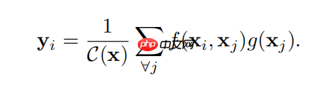
上式中，一文搞懂卷积网络之四（空间注意力Non-local） - php中文网计算特征图x中代表i,j两个点相关关系的标量。（A pairwise func-tion f computes a scalar (representing relationship such as affinity) between i and all j.）计算的是代表特征图x中j点的值。（The unary function g computes a representation of the input signal at the position j.）最后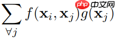一文搞懂卷积网络之四（空间注意力Non-local） - php中文网计算出的特征图所有点之间的响应值通过进行标准化。（The response is normalized by a factor C(x).）

如文章中所说，这种 Non-local 机制是一种通用（generic）的注意力实现方法，所以上式中的一文搞懂卷积网络之四（空间注意力Non-local） - php中文网可以使用不同的方式实现相关性计算。这就有了通过 Embedded Gaussion、Vanilla Gaussion、Dot product 和 Concatenation 几种方式实现的 Non-local 模块。后面我们会实现其中的前三种结构，并测试其对网络性能的提升作用。

文章地址：https://arxiv.org/abs/1711.07971
作者源码地址：https://github.com/facebookresearch/video-nonlocal-net

三、Non-local 结构的实现

文章中对 Non-local 模块的结构总结如下图：

一文搞懂卷积网络之四（空间注意力Non-local） - php中文网

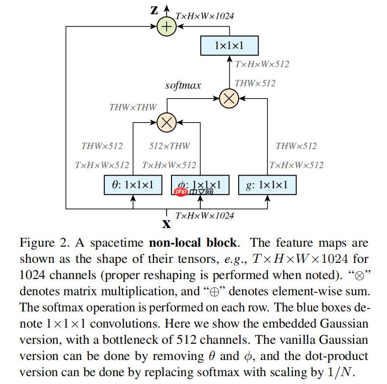
如上图所示，先将输入的特征图降维（降到1维）后逐次嵌入（embed）到 theta、phi 和 g 三个向量中。然后，将向量 theta 和向量 phi 的转置相乘，做 softmax 激活后再与向量 g 相乘。最后，再将这个 Non-local 操作包裹一层，这通过一个1×1的卷积核和一个跨层连接实现，以方便嵌入此注意力模块到现有系统中(We wrap the non-local operation in Eq.(1) into a non-local block that can be incorporated into many existing architectures.)。

在实现的过程中还要注意几个地方：

再将降维后的特征图嵌入三个向量中时，可以进行通道缩减（如上图所示缩减比例为一半），然后在最后经过1×1卷积时再升回来。这样类似 BottleNeck 的结构可以节省大约一半参数。(We set the number of channels represented by Wg, Wθ, and Wφ to be half of the number of channels in x. This follows the bottleneck design of [21] and reduces the computation of a block by about a half.)
模块最后的1×1卷积后面加了一个 BN 层，这个 BN 层的放大系数（也就是权重参数）全部初始化为 0，以确保此模块的初始状态为恒等映射，使得其可以被插入到使用预训练权重的模型中去。(We add a BN layer right after the last 1×1×1 layer that represents Wz; we do not add BN to other layers in a non-local block. The scale parameter of this BN layer is initialized as zero, following [17]. This ensures that the initial state of the entire non-local block is an identity mapping, so it can be inserted into any pre-trained networks while maintaining its initial behavior.)
文章中实现的是视频分类的 Non-local 模块，使用的是 T×H×W 的3D卷积，我们这里实现图片分类的 Non-local 模块时要去掉卷积的 T（时间）维度，采用2D卷积。

实现 Non-local 模块前先做好依赖项导入、参数设置、数据集处理等准备工作：

In [5]

import paddleimport paddle.nn as nnfrom paddle.io import DataLoaderimport numpy as npimport osimport paddle.vision.transforms as Tfrom paddle.vision.datasets import Cifar10import matplotlib.pyplot as plt
%matplotlib inlineimport warnings
warnings.filterwarnings("ignore", category=Warning) # 过滤报警信息BATCH_SIZE = 32PIC_SIZE = 96EPOCH_NUM = 30CLASS_DIM = 10PLACE = paddle.CPUPlace() # 在cpu上训练# PLACE = paddle.CUDAPlace(0)  # 在gpu上训练# 数据集处理transform = T.Compose([
    T.Resize(PIC_SIZE),
    T.Transpose(),
    T.Normalize([127.5, 127.5, 127.5], [127.5, 127.5, 127.5]),
])
train_dataset = Cifar10(mode='train', transform=transform)
val_dataset = Cifar10(mode='test', transform=transform)
train_loader = DataLoader(train_dataset, places=PLACE, shuffle=True, batch_size=BATCH_SIZE, drop_last=True, num_workers=0, use_shared_memory=False)
valid_loader = DataLoader(val_dataset, places=PLACE, shuffle=False, batch_size=BATCH_SIZE, drop_last=True, num_workers=0, use_shared_memory=False)def save_show_pics(pics, file_name='tmp', save_path='./output/pics/', save_root_path='./output/'):
    if not os.path.exists(save_root_path):
        os.makedirs(save_root_path)    if not os.path.exists(save_path):
        os.makedirs(save_path)
    shape = pics.shape
    pic = pics.transpose((0,2,3,1)).reshape([-1,8,PIC_SIZE,PIC_SIZE,3])
    pic = np.concatenate(tuple(pic), axis=1)
    pic = np.concatenate(tuple(pic), axis=1)
    pic = (pic + 1.) / 2.
    plt.imsave(save_path+file_name+'.jpg', pic)    # plt.figure(figsize=(8,8), dpi=80)
    plt.imshow(pic)
    plt.xticks([])
    plt.yticks([])
    plt.show()

test_loader = DataLoader(train_dataset, places=PLACE, shuffle=True, batch_size=BATCH_SIZE, drop_last=True, num_workers=0, use_shared_memory=False)
data, label = next(test_loader())
save_show_pics(data.numpy())

登录后复制

<Figure size 432x288 with 1 Axes>

登录后复制

1.Embedded Gaussian 实现 Non-local 模块

如以上所描述的，我们实现的就是最常用的用 Embedded Gaussian 实现的 Non-local 模块：

In [ ]

class EmbeddedGaussion(nn.Layer):
    def __init__(self, shape):
        super(EmbeddedGaussion, self).__init__()

        input_dim = shape[1]

        self.theta = nn.Conv2D(input_dim, input_dim // 2, 1)
        self.phi = nn.Conv2D(input_dim, input_dim // 2, 1)
        self.g = nn.Conv2D(input_dim, input_dim // 2, 1)

        self.conv = nn.Conv2D(input_dim // 2, input_dim, 1)
        self.bn = nn.BatchNorm2D(input_dim, weight_attr=paddle.ParamAttr(initializer=nn.initializer.Constant(0)))    def forward(self, x):
        shape = x.shape

        theta = paddle.flatten(self.theta(x), start_axis=2, stop_axis=-1)
        phi = paddle.flatten(self.phi(x), start_axis=2, stop_axis=-1)
        g = paddle.flatten(self.g(x), start_axis=2, stop_axis=-1)

        non_local = paddle.matmul(theta, phi, transpose_y=True)
        non_local = nn.functional.softmax(non_local)
        non_local = paddle.matmul(non_local, g)
        non_local = paddle.reshape(non_local, [shape[0], shape[1] // 2, shape[2], shape[3]])
        non_local = self.bn(self.conv(non_local))        return non_local + x

nl = EmbeddedGaussion([16, 16, 8, 8])
x = paddle.to_tensor(np.random.uniform(-1, 1, [16, 16, 8, 8]).astype('float32'))
y = nl(x)print(y.shape)

登录后复制

[16, 16, 8, 8]

登录后复制

2.Vanilla Gaussian 实现 Non-local 模块

Embedded Gaussian 实现的 Non-local 模块如果去掉特征图嵌入向量 theta 和向量 g 的操作，就是普通的用 Vanilla Gaussian 实现的 Non-local 版本了。当然，没有了前面的1×1卷积，通道缩减也就无从谈起了。

In [ ]

class VanillaGaussion(nn.Layer):
    def __init__(self, shape):
        super(VanillaGaussion, self).__init__()

        input_dim = shape[1]

        self.g = nn.Conv2D(input_dim, input_dim, 1)

        self.conv = nn.Conv2D(input_dim, input_dim, 1)
        self.bn = nn.BatchNorm(input_dim)    def forward(self, x):
        shape = x.shape

        theta = paddle.flatten(x, start_axis=2, stop_axis=-1)
        phi = paddle.flatten(x, start_axis=2, stop_axis=-1)
        g = paddle.flatten(self.g(x), start_axis=2, stop_axis=-1)

        non_local = paddle.matmul(theta, phi, transpose_y=True)
        non_local = nn.functional.softmax(non_local)
        non_local = paddle.matmul(non_local, g)
        non_local = paddle.reshape(non_local, shape)
        non_local = self.bn(self.conv(non_local))        return non_local + x

nl = VanillaGaussion([16, 16, 8, 8])
x = paddle.to_tensor(np.random.uniform(-1, 1, [16, 16, 8, 8]).astype('float32'))
y = nl(x)print(y.shape)

登录后复制

[16, 16, 8, 8]

登录后复制

3.Dot Production 实现 Non-local 模块

Embedded Gaussian 实现 Non-local 的模块如果去掉 SoftMax 激活操作，通过除以 N（N 为特征图的位置数量）进行缩放代替，就是 Dot Production 实现的 Non-local 版本了。

神卷标书

神卷标书，专注于AI智能标书制作、管理与咨询服务，提供高效、专业的招投标解决方案。支持一站式标书生成、模板下载，助力企业轻松投标，提升中标率。

查看详情

In [ ]

class DotProduction(nn.Layer):
    def __init__(self, shape):
        super(DotProduction, self).__init__()

        input_dim = shape[1]

        self.theta = nn.Conv2D(input_dim, input_dim // 2, 1)
        self.phi = nn.Conv2D(input_dim, input_dim // 2, 1)
        self.g = nn.Conv2D(input_dim, input_dim // 2, 1)

        self.conv = nn.Conv2D(input_dim // 2, input_dim, 1)
        self.bn = nn.BatchNorm(input_dim)    def forward(self, x):
        shape = x.shape

        theta = paddle.flatten(self.theta(x), start_axis=2, stop_axis=-1)
        phi = paddle.flatten(self.phi(x), start_axis=2, stop_axis=-1)
        g = paddle.flatten(self.g(x), start_axis=2, stop_axis=-1)

        non_local = paddle.matmul(theta, phi, transpose_y=True)
        non_local = non_local / shape[2]
        non_local = paddle.matmul(non_local, g)
        non_local = paddle.reshape(non_local, [shape[0], shape[1] // 2, shape[2], shape[3]])
        non_local = self.bn(self.conv(non_local))        return non_local + x

nl = DotProduction([16, 16, 8, 8])
x = paddle.to_tensor(np.random.uniform(-1, 1, [16, 16, 8, 8]).astype('float32'))
y = nl(x)print(y.shape)

登录后复制

[16, 16, 8, 8]

登录后复制

四、Non-local 的运行对比效果

下面我们就来实验下刚才实现的三个版本的 Non-local 模块的效果。原文是在视频分类数据集上做的实验，这里我们用 Paddle 内置的 Cifar10 图片分类数据集做下实验。

1.运行 ResNet18 基线版本

在 ResNet18 模型结构上加上一个残差块作为基线版本，后面的 Non-local 模块就替换这个残差块。这样能确认效果的提升来自 Non-Local 结构，而非增加的参数。

In [ ]

class Residual(nn.Layer):
    def __init__(self, num_channels, num_filters, use_1x1conv=False, stride=1):
        super(Residual, self).__init__()
        self.use_1x1conv = use_1x1conv
        model = [
            nn.Conv2D(num_channels, num_filters, 3, stride=stride, padding=1),
            nn.BatchNorm2D(num_filters),
            nn.ReLU(),
            nn.Conv2D(num_filters, num_filters, 3, stride=1, padding=1),
            nn.BatchNorm2D(num_filters),
        ]
        self.model = nn.Sequential(*model)        if use_1x1conv:
            model_1x1 = [nn.Conv2D(num_channels, num_filters, 1, stride=stride)]
            self.model_1x1 = nn.Sequential(*model_1x1)    def forward(self, X):
        Y = self.model(X)        if self.use_1x1conv:
            X = self.model_1x1(X)        return paddle.nn.functional.relu(X + Y)class ResnetBlock(nn.Layer):
    def __init__(self, num_channels, num_filters, num_residuals, first_block=False):
        super(ResnetBlock, self).__init__()
        model = []        for i in range(num_residuals):            if i == 0:                if not first_block:
                    model += [Residual(num_channels, num_filters, use_1x1conv=True, stride=2)]                else:
                    model += [Residual(num_channels, num_filters)]            else:
                model += [Residual(num_filters, num_filters)]
        self.model = nn.Sequential(*model)    def forward(self, X):
        return self.model(X)class ResNet(nn.Layer):
    def __init__(self, num_classes=10):
        super(ResNet, self).__init__()
        model = [
            nn.Conv2D(3, 64, 7, stride=2, padding=3),
            nn.BatchNorm2D(64),
            nn.ReLU(),
            nn.MaxPool2D(kernel_size=3, stride=2, padding=1)
        ]

        model += [
            ResnetBlock(64, 64, 2, first_block=True),
            ResnetBlock(64, 128, 2),            # ResnetBlock(128, 256, 2),
            ResnetBlock(128, 256, 2 + 1),
            ResnetBlock(256, 512, 2)
        ]

        model += [
            nn.AdaptiveAvgPool2D(output_size=1),
            nn.Flatten(start_axis=1, stop_axis=-1),
            nn.Linear(512, num_classes),
        ]
        self.model = nn.Sequential(*model)    def forward(self, X):
        Y = self.model(X)        return Y# 模型定义model = paddle.Model(ResNet(num_classes=CLASS_DIM))# 设置训练模型所需的optimizer, loss, metricmodel.prepare(
    paddle.optimizer.Adam(learning_rate=1e-4, parameters=model.parameters()),
    paddle.nn.CrossEntropyLoss(),
    paddle.metric.Accuracy(topk=(1, 5)))# 启动训练、评估model.fit(train_loader, valid_loader, epochs=EPOCH_NUM, log_freq=500, 
    callbacks=paddle.callbacks.VisualDL(log_dir='./log/BLResNet18+1'))

登录后复制

The loss value printed in the log is the current step, and the metric is the average value of previous step.
Epoch 1/30

登录后复制

2.测试加入 Non-local 模块的版本

分别测试用 Embedded Gaussian、Vanilla Gaussian 和 Dot Production 方法实现的 Non-local 模块的效果。

In [ ]

class Residual(nn.Layer):
    def __init__(self, num_channels, num_filters, use_1x1conv=False, stride=1):
        super(Residual, self).__init__()
        self.use_1x1conv = use_1x1conv
        model = [
            nn.Conv2D(num_channels, num_filters, 3, stride=stride, padding=1),
            nn.BatchNorm2D(num_filters),
            nn.ReLU(),
            nn.Conv2D(num_filters, num_filters, 3, stride=1, padding=1),
            nn.BatchNorm2D(num_filters),
        ]
        self.model = nn.Sequential(*model)        if use_1x1conv:
            model_1x1 = [nn.Conv2D(num_channels, num_filters, 1, stride=stride)]
            self.model_1x1 = nn.Sequential(*model_1x1)    def forward(self, X):
        Y = self.model(X)        if self.use_1x1conv:
            X = self.model_1x1(X)        return paddle.nn.functional.relu(X + Y)class ResnetBlock(nn.Layer):
    def __init__(self, num_channels, num_filters, num_residuals, first_block=False):
        super(ResnetBlock, self).__init__()
        model = []        for i in range(num_residuals):            if i == 0:                if not first_block:
                    model += [Residual(num_channels, num_filters, use_1x1conv=True, stride=2)]                else:
                    model += [Residual(num_channels, num_filters)]            else:
                model += [Residual(num_filters, num_filters)]
        self.model = nn.Sequential(*model)    def forward(self, X):
        return self.model(X)class ResNetNonLocal(nn.Layer):
    def __init__(self, num_classes=10):
        super(ResNetNonLocal, self).__init__()
        model = [
            nn.Conv2D(3, 64, 7, stride=2, padding=3),
            nn.BatchNorm2D(64),
            nn.ReLU(),
            nn.MaxPool2D(kernel_size=3, stride=2, padding=1)
        ]

        model += [
            ResnetBlock(64, 64, 2, first_block=True),
            ResnetBlock(64, 128, 2),
            ResnetBlock(128, 256, 2),
            EmbeddedGaussion([BATCH_SIZE, 256, 14, 14]),            # VanillaGaussion([BATCH_SIZE, 256, 14, 14]),
            # DotProduction([BATCH_SIZE, 256, 14, 14]),
            # # EmbeddedGaussionNoBottleNeck([BATCH_SIZE, 256, 14, 14]),
            ResnetBlock(256, 512, 2),
        ]

        model += [
            nn.AdaptiveAvgPool2D(output_size=1),
            nn.Flatten(start_axis=1, stop_axis=-1),
            nn.Linear(512, num_classes),
        ]
        self.model = nn.Sequential(*model)    def forward(self, X):
        Y = self.model(X)        return Y# 模型定义model = paddle.Model(ResNetNonLocal(num_classes=CLASS_DIM))# 设置训练模型所需的optimizer, loss, metricmodel.prepare(
    paddle.optimizer.Adam(learning_rate=1e-4, parameters=model.parameters()),
    paddle.nn.CrossEntropyLoss(),
    paddle.metric.Accuracy(topk=(1, 5)))# 启动训练、评估model.fit(train_loader, valid_loader, epochs=EPOCH_NUM, log_freq=500, 
    callbacks=paddle.callbacks.VisualDL(log_dir='./log/EmbeddedGaussion'))# model.fit(train_loader, valid_loader, epochs=EPOCH_NUM, log_freq=500, #     callbacks=paddle.callbacks.VisualDL(log_dir='./log/VanillaGaussion'))# model.fit(train_loader, valid_loader, epochs=EPOCH_NUM, log_freq=500, #     callbacks=paddle.callbacks.VisualDL(log_dir='./log/DotProduction'))

登录后复制

The loss value printed in the log is the current step, and the metric is the average value of previous step.
Epoch 1/30

登录后复制

上面的代码需要运行三次，每次需要注释掉 ResNetNonLocal 类的 forward() 方法里不同版本的 Non-local 模块，并且在 model.fit 写入VisualDL 的 log 文件时用不同的名称。

接下来，我们对比下运行结果的验证集准确率：

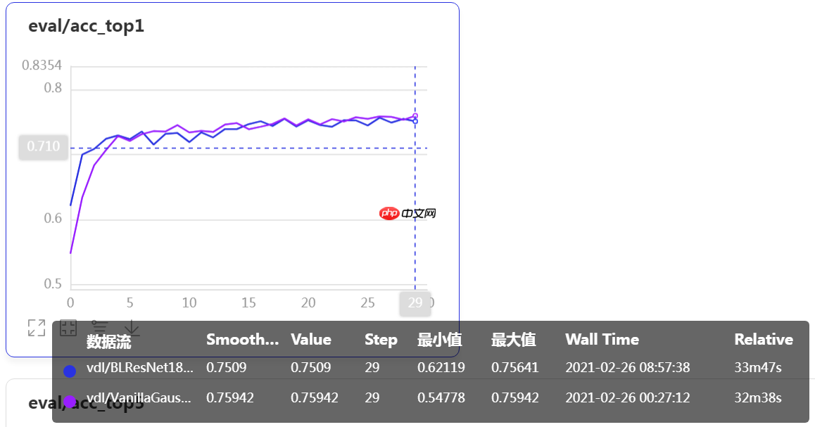1)测试 Vanilla Gaussian 版本 Non-local 模块

一文搞懂卷积网络之四（空间注意力Non-local） - php中文网上图中，蓝色线为 ResNet18 加一个残差块的基线版本的验证集准确率曲线，紫色线为加入Vanilla Gaussian 版本 Non-local 模块后模型的验证集准确率曲线。改进的模型准曲率提高了0.3%。

2)测试 Dot Production 版本 Non-local 模块

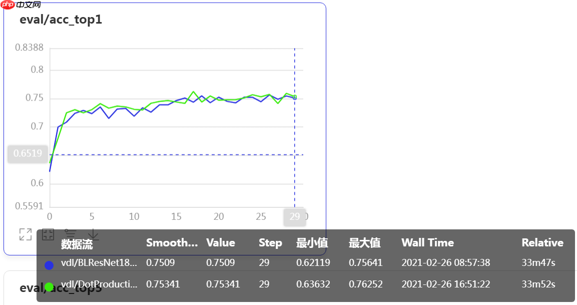一文搞懂卷积网络之四（空间注意力Non-local） - php中文网蓝色线仍为基线模型准确率，绿线为加入Dot Production 版本 Non-local 模块后模型的准确率。改进的模型准曲率提高了0.6%。

3)测试 Embedded Gaussian 版本 Non-local 模块

最后来测试下“顶配”版本的。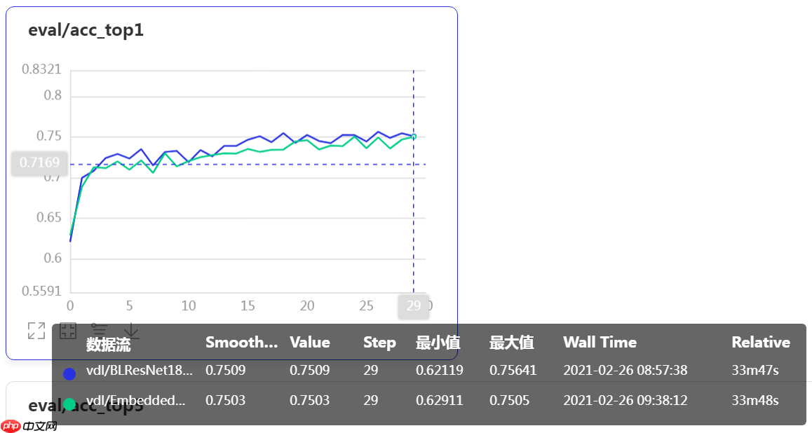一文搞懂卷积网络之四（空间注意力Non-local） - php中文网仍然蓝色线为基线模型数据...我去，这么好的装备怎么出现了这么差的结果，加了 Embedded Gaussian 版本 Non-local 模块的模型精度甚至低于基线模型的精度，这是肿么回事？！&@%

一顿修改猛如虎之后（换模型结构、换数据集、换数据增强、换超参），似乎找到一点儿线索。

4)测试不缩减通道数的 Embedded Gaussian 版本 Non-local 模块

在下面这个 Embedded Gaussian 版本 Non-local 模块中，我们不在1×1卷积上采用类似 BottleNeck 的结构缩减通道数。

In [4]

class EmbeddedGaussionNoBottleNeck(nn.Layer):
    def __init__(self, shape):
        super(EmbeddedGaussionNoBottleNeck, self).__init__()

        input_dim = shape[1]

        self.theta = nn.Conv2D(input_dim, input_dim, 1)
        self.phi = nn.Conv2D(input_dim, input_dim, 1)
        self.g = nn.Conv2D(input_dim, input_dim, 1)

        self.conv = nn.Conv2D(input_dim, input_dim, 1)
        self.bn = nn.BatchNorm(input_dim)    def forward(self, x):
        shape = x.shape

        theta = paddle.flatten(self.theta(x), start_axis=2, stop_axis=-1)
        phi = paddle.flatten(self.phi(x), start_axis=2, stop_axis=-1)
        g = paddle.flatten(self.g(x), start_axis=2, stop_axis=-1)

        non_local = paddle.matmul(theta, phi, transpose_y=True)
        non_local = nn.functional.softmax(non_local)
        non_local = paddle.matmul(non_local, g)
        non_local = paddle.reshape(non_local, shape)
        non_local = self.bn(self.conv(non_local))        return non_local + x

nl = EmbeddedGaussionNoBottleNeck([16, 16, 8, 8])
x = paddle.to_tensor(np.random.uniform(-1, 1, [16, 16, 8, 8]).astype('float32'))
y = nl(x)print(y.shape)

登录后复制

[16, 16, 8, 8]

登录后复制

训练后与基线模型对照下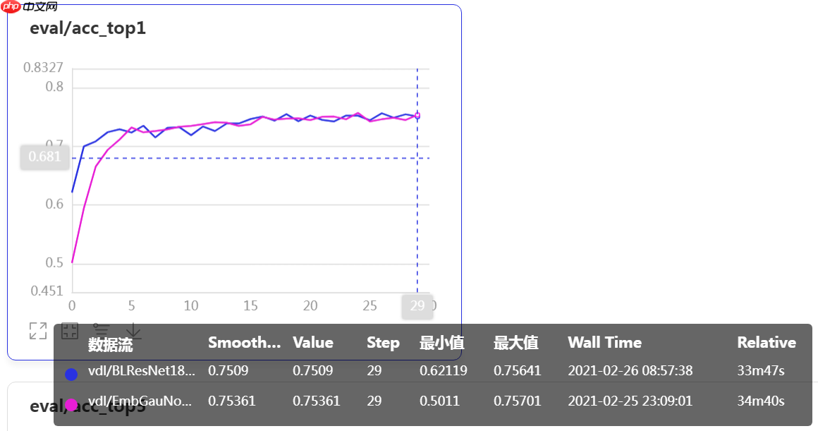：一文搞懂卷积网络之四（空间注意力Non-local） - php中文网蓝色为基线模型版本曲线。在增加了 Non-local 模块的宽度后，性能和基线版本差不多，虽然没有 Vanilla Gaussian 和 Dot Production 实现的版本提升的精度多，但已经比原来的降低通道数的 Embedded Gaussian 版本好了不少。

五、总结

各种消融实验完毕，总结学习体会。

无论是在 Non-local 结构还是在 ResNet 的残差块中，BottleNeck 结构只适合在深层网络中用于减少参数量。在原版的 ResNet 的结构里，也只有 50 层以上的配置才会使用 BottleNeck 结构。这也解释了在前面项目实验（ResNet一族）中，后面出的一些 ResNet 魔该版本，基本都是在 50 层以上挑战大规模数据集。这些改动都是建立在 BottelNeck 基础上的，所以才用在我们的浅层网络中会效果欠佳。这可能是因为深层的网络中，被激活的神经元更稀疏，才能通过 BottelNeck 使用更窄的网络来减少参数。而在较浅的网络中，网络的宽度对性能影响还是挺大的。
Non-local 模块的使用位置是很重要的，在模型的不同层加入注意力模块的效果大相径庭，在不同的数据集上效果也不同（在224×224尺寸的OxfordFlower102 和 CalTech201 数据集上，找这个合适的位置更难，放弃了。我想也许作者当年在视频数据集上做实验也是有原因的吧。），加注意力模块的位置不好反而会使模型性能下降。有的信息说注意力快适合用在前面的层，但是在这个实验里，还是放在后面用来提取更大粒度特征图的位置相关特征时效果更好。

以上就是一文搞懂卷积网络之四（空间注意力Non-local）的详细内容，更多请关注php中文网其它相关文章！