本文介绍基于PaddleDetection的情绪识别项目。使用Fer2013数据集,先预处理数据,构建VGG模型训练,经300轮迭代精度达62.16%。后用ResNet34模型优化,准确率提升至64.85%。还利用PaddleDetection进行人脸识别,将表情识别结果标注在人脸框上,完成情绪识别全流程。
☞☞☞AI 智能聊天, 问答助手, AI 智能搜索, 免费无限量使用 DeepSeek R1 模型☜☜☜

基于PaddleDetection的情绪识别
一、项目背景
表情识别(facialexpression recognition, FER)是计算机理解人类情感的一个重要方向,也是人机交互的一个重要方面。表情识别是指从静态照片或视频序列中选择出表情状态,从而确定对人物的情绪与心理变化。20世纪70年代的美国心理学家Ekman和Friesen通过大量实验,定义了人类六种基本表情:快乐,气愤,惊讶,害怕,厌恶和悲伤,除此之外后续的分类任务大多增添了一个中性表情。人脸表情识别(FER)在人机交互和情感计算中有着广泛的研究前景,包括人机交互、情绪分析、智能安全等。
PaddleDetection为基于飞桨PaddlePaddle的端到端目标检测套件,内置30+模型算法及250+预训练模型,覆盖目标检测、实例分割、跟踪、关键点检测等方向,其中包括服务器端和移动端高精度、轻量级产业级SOTA模型、冠军方案和学术前沿算法,并提供配置化的网络模块组件、十余种数据增强策略和损失函数等高阶优化支持和多种部署方案,在打通数据处理、模型开发、训练、压缩、部署全流程的基础上,提供丰富的案例及教程,加速算法产业落地应用。
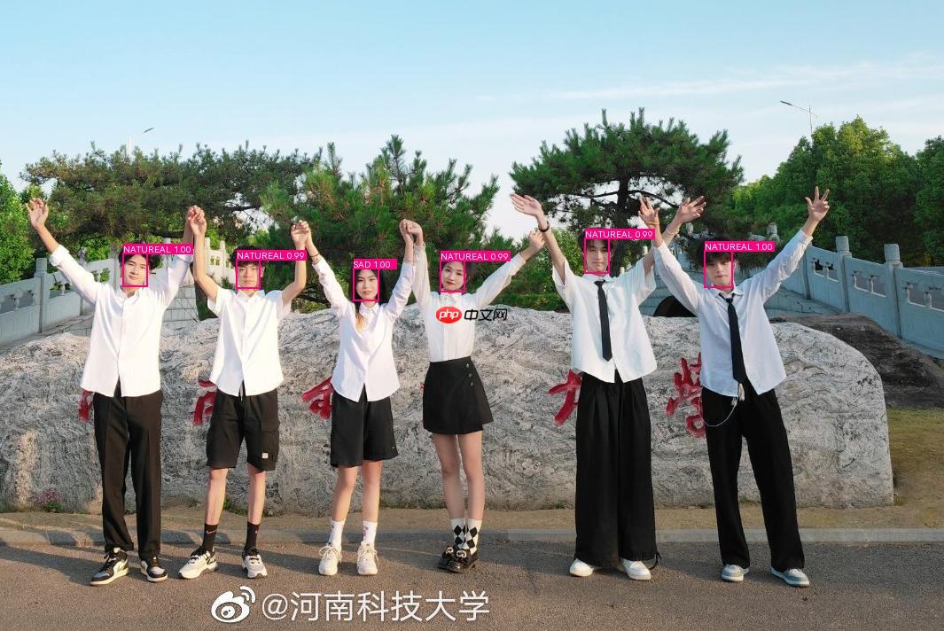
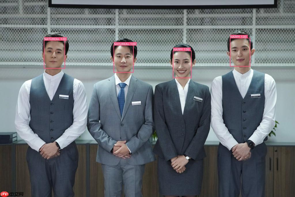
效果如下图所示:
本项目利用飞桨框架搭建VGG网络,可优化后改使用ResNet34网络,基于fer2013数据集实现情绪分析
主要技术点有:
- 使用PaddleDetection提供的目标检测模型,将人物信息提取出来。
- 训练人脸检测模型,对提取出的人物信息进行人脸检测,判断能否进行情绪识别。
- 将识别出来的可以进行情绪识别的人脸输入进VGG分类模型,通过分析表情和背景识别出人物情绪。
- 最后将识别出来的表情结合PaddleDetection标注在图片人脸上。
二、环境和数据集的准备
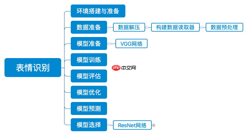
表情识别的整体流程如下:
2.1 数据集介绍
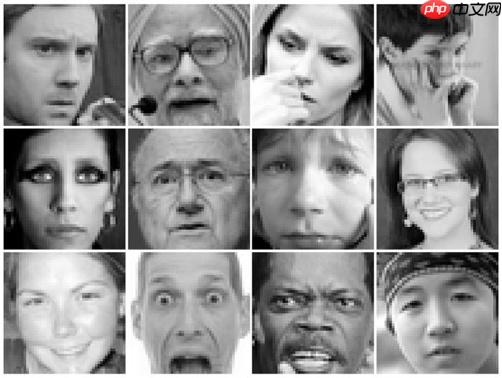
本次实验的使用的数据集为Fer2013,它于2013年国际机器学习会议(ICML)上推出,并成为比较表情识别模型性能的基准之一,同时也作为了2013年Kaggle人脸识别比赛的数据。Fer2013包含28709张训练集图像、3589张公开测试集图像和3589张私有测试集图像,每张图像为4848大小的灰度图片,如下图所示。Fer2013数据集中由有生气(angry)、厌恶(disgust)、恐惧(fear)、开心(happy)、难过(sad)、惊讶(surprise)和中性(neutral)七个类别组成。由于这个数据集大多是通过爬虫在互联网上进行爬取所得,因此存在一定的误差性。
2.2 数据集准备
将数据集的压缩包解压到emotic文件夹中:
%cd /home/aistudio
!unzip -oq data/data150581/archive.zip -d ./emotic
/home/aistudio
将数据集整理成以文件名表示类别的形式
import osimport cv2import tqdmdef make_new_dir(root_dir, tag, save_dir):
    img_root = os.path.join(root_dir, tag)
    img_dir_list = os.listdir(img_root)    if not os.path.isdir(save_dir):
        os.mkdir(save_dir)    print(img_dir_list)    for img_dir in tqdm.tqdm(img_dir_list):
        img_folder = os.path.join(img_root, img_dir)
        img_list = [f for f in os.listdir(img_folder) if f.endswith('.jpg')]
        name_first = img_dir[:2].upper()        for index, filename in enumerate(img_list):
            img = cv2.imread(os.path.join(img_folder, filename), -1)
            save_name = name_first+"{0:0>5}.jpg".format(index)
            cv2.imwrite(os.path.join(save_dir, save_name), img)
root_dir = r"emotic"save_dir = r"train"make_new_dir(root_dir, "train", save_dir) # 制作训练集
0%| | 0/7 [00:00
['surprise', 'sad', 'fear', 'disgust', 'neutral', 'happy', 'angry']
100%|██████████| 7/7 [00:04<00:00, 1.73it/s]
root_dir = r"emotic"save_dir = r"test"make_new_dir(root_dir, "test", save_dir) # 制作测试集
14%|█▍ | 1/7 [00:00<00:00, 8.58it/s]
['surprise', 'sad', 'fear', 'disgust', 'neutral', 'happy', 'angry']
29%|██▊ | 2/7 [00:00<00:00, 7.74it/s]
100%|██████████| 7/7 [00:00<00:00, 7.33it/s]
# 随机移动10%数量的图像到val文件夹中import shutilimport osimport randomdef move2newDir(inputFolder, saveFolder):
    filenames = [f for f in os.listdir(inputFolder) if f.endswith('.jpg')]
    random.shuffle(filenames)
    num_val = int(0.1*len(filenames))    if not os.path.isdir(saveFolder):
        os.mkdir(saveFolder)
    for index, filename in enumerate(filenames):
        src = os.path.join(inputFolder,filename)
        dst = os.path.join(saveFolder,filename)
        shutil.move(src, dst)        if index == num_val:            break
inputFolder = r"train"saveFolder = r"val"move2newDir(inputFolder, saveFolder)
2.3 查看数据集
查看数据集图片:train/val/test文件夹里包含7种表情类型图片 以NE,HA,SU作为名称前缀的图片分别代表neutral,happy,surprised三种表情
import osimport numpy as npimport matplotlib.pyplot as plt
%matplotlib inlinefrom PIL import Image#选取 test文件夹 作为图片路径DATADIR = 'test' # 文件名以N开头的是普通表情的图片,以H开头的是高兴图片,以S开头的是惊讶的图片#file0-3选取了三个文件夹里的三个表情file0 = 'NE00127.jpg'file1 = 'HA00453.jpg'file2 = 'SU00224.jpg'# 读取图片img0 = Image.open(os.path.join(DATADIR, file0))
img0 = np.array(img0)
img1 = Image.open(os.path.join(DATADIR, file1))
img1 = np.array(img1)
img2 = Image.open(os.path.join(DATADIR, file2))
img2 = np.array(img2)# 画出读取的图片plt.figure(figsize=(16, 8))

f = plt.subplot(131)
f.set_title('0', fontsize=20)
plt.imshow(img0)

f = plt.subplot(132)
f.set_title('1', fontsize=20)
plt.imshow(img1)

f = plt.subplot(133)
f.set_title('2', fontsize=20)
plt.imshow(img2)#plt展示出三个表情plt.show()
三、数据预处理
3.1 定义数据读取器
使用OpenCV从磁盘读入图片,将每张图缩放到224×224大小,并且将像素值调整到[−1,1][-1, 1][−1,1]之间,代码如下所示:
import cv2import randomimport numpy as npimport os# 对读入的图像数据进行预处理def transform_img(img):
    # 将图片尺寸缩放道 224x224
    img = cv2.resize(img, (224, 224))    # 读入的图像数据格式是[H, W, C]
    # 使用转置操作将其变成[C, H, W]
    img = np.transpose(img, (2,0,1))
    img = img.astype('float32')    # 将数据范围调整到[-1.0, 1.0]之间
    img = img / 255.
    img = img * 2.0 - 1.0
    return img# 定义训练集数据读取器def data_loader(datadir, batch_size=20, mode = 'train'):
    # 将datadir目录下的文件列出来,每条文件都要读入
    filenames = os.listdir(datadir)    def reader():
        if mode == 'train':            # 训练时随机打乱数据顺序
            random.shuffle(filenames)
        batch_imgs = []
        batch_labels = []        for name in filenames:
            filepath = os.path.join(datadir, name)
            img = cv2.imread(filepath)
            img = transform_img(img)            #依次读取每张图片的名称首字母用于标记标签
            # 7类表情 'sad', 'disgust', 'happy', 'fear', 'surprise', 'neutral', 'angry'
            # SA开头表示sad表情用0标签
            # DI开头表示disgust表情用1标签
            # HA开头表示happy表情用2标签,以此类推
            if name[:2] == 'SA':
                label = 0
            elif name[:2] == 'DI':
                label = 1
            elif name[:2] == 'HA':
                label = 2
            elif name[:2] == 'FE':
                label = 3
            elif name[:2] == 'SU':
                label = 4
            elif name[:2] == 'NE':
                label = 5
            elif name[:2] == 'AN':
                label = 6
            else:                raise('Not excepted file name')            # 每读取一个样本的数据,就将其放入数据列表中
            batch_imgs.append(img)
            batch_labels.append(label)            if len(batch_imgs) == batch_size:                # 当数据列表的长度等于batch_size的时候,
                # 把这些数据当作一个mini-batch,并作为数据生成器的一个输出
                imgs_array = np.array(batch_imgs).astype('float32')
                labels_array = np.array(batch_labels).reshape(-1, 1)                yield imgs_array, labels_array
                batch_imgs = []
                batch_labels = []        if len(batch_imgs) > 0:            # 剩余样本数目不足一个batch_size的数据,一起打包成一个mini-batch
            imgs_array = np.array(batch_imgs).astype('float32')
            labels_array = np.array(batch_labels).reshape(-1, 1)            yield imgs_array, labels_array    return reader# 定义验证集数据读取器def valid_data_loader(datadir, batch_size=20, mode='valid'):
    filenames = os.listdir(datadir)    def reader():
        batch_imgs = []
        batch_labels = []            # 根据图片文件名加载图片,并对图像数据作预处理
        for name in filenames:
            filepath = os.path.join(datadir, name)            # 每读取一个样本的数据,就将其放入数据列表中
            img = cv2.imread(filepath)
            img = transform_img(img)            #根据名称判断标签
            if name[:2] == 'SA':
                label = 0
            elif name[:2] == 'DI':
                label = 1
            elif name[:2] == 'HA':
                label = 2
            elif name[:2] == 'FE':
                label = 3
            elif name[:2] == 'SU':
                label = 4
            elif name[:2] == 'NE':
                label = 5
            elif name[:2] == 'AN':
                label = 6
            else:                raise('Not excepted file name')            # 每读取一个样本的数据,就将其放入数据列表中
            batch_imgs.append(img)
            batch_labels.append(label)            if len(batch_imgs) == batch_size:                # 当数据列表的长度等于batch_size的时候,
                # 把这些数据当作一个mini-batch,并作为数据生成器的一个输出
                imgs_array = np.array(batch_imgs).astype('float32')
                labels_array = np.array(batch_labels).reshape(-1, 1)                yield imgs_array, labels_array
                batch_imgs = []
                batch_labels = []        if len(batch_imgs) > 0:            # 剩余样本数目不足一个batch_size的数据,一起打包成一个mini-batch
            imgs_array = np.array(batch_imgs).astype('float32')
            labels_array = np.array(batch_labels).reshape(-1, 1)            yield imgs_array, labels_array    return reader
3.2 校验数据
将train文件夹中的数据传入到数据读取器,再输出处理后的数据格式
# 查看数据形状DATADIR = 'train'train_loader = data_loader(DATADIR,batch_size=20, mode='train')
data_reader = train_loader()
data = next(data_reader) #返回迭代器的下一个项目给data# 输出表示: 图像数据(batchsize,通道数,224*224)标签(batchsize,标签维度)print("train mode's shape:")print("data[0].shape = %s, data[1].shape = %s" %(data[0].shape, data[1].shape))

eval_loader = data_loader(DATADIR,batch_size=20, mode='eval')
data_reader = eval_loader()
data = next(data_reader)# 输出表示: 图像数据(batchsize,通道数,224*224)标签(batchsize,标签维度)print("eval mode's shape:")print("data[0].shape = %s, data[1].shape = %s" %(data[0].shape, data[1].shape))
train mode's shape:
data[0].shape = (20, 3, 224, 224), data[1].shape = (20, 1)
eval mode's shape:
data[0].shape = (20, 3, 224, 224), data[1].shape = (20, 1)
四、VGG模型实现
4.1 VGG模型介绍
本案例中我们使用VGG网络进行表情识别,首先我们来了解一下VGG模型。 VGG是当前最流行的CNN模型之一,2014年由Simonyan和Zisserman发表在ICLR 2015会议上的论文《Very Deep Convolutional Networks For Large-scale Image Recognition》提出,其命名来源于论文作者所在的实验室Visual Geometry Group。VGG设计了一种大小为3x3的小尺寸卷积核和池化层组成的基础模块,通过堆叠上述基础模块构造出深度卷积神经网络,该网络在图像分类领域取得了不错的效果,在大型分类数据集ILSVRC上,VGG模型仅有6.8% 的top-5 test error 。VGG模型一经推出就很受研究者们的欢迎,因为其网络结构的设计合理,总体结构简明,且可以适用于多个领域。VGG的设计为后续研究者设计模型结构提供了思路。
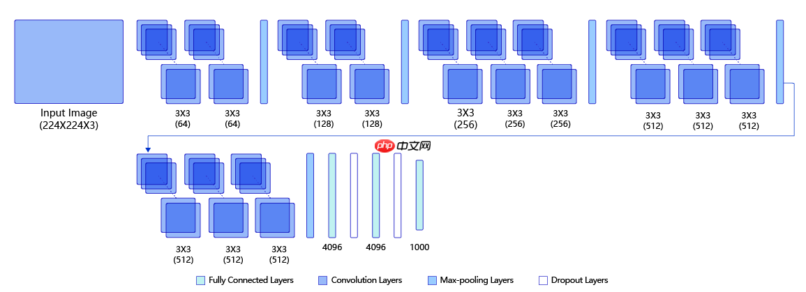
下图是VGG-16的网络结构示意图,一共包含13层卷积和3层全连接层。VGG网络使用3×3的卷积层和池化层组成的基础模块来提取特征,三层全连接层放在网络的最后组成分类器,最后一层全连接层的输出即为分类的预测。 在VGG中每层卷积将使用ReLU作为激活函数,在全连接层之后添加dropout来抑制过拟合。使用小的卷积核能够有效地减少参数的个数,使得训练和测试变得更加有效。比如如果我们想要得到感受野为5的特征图,最直接的方法是使用5×5的卷积层,但是我们也可以使用两层3×3卷积层达到同样的效果,并且只需要更少的参数。另外由于卷积核比较小,我们可以堆叠更多的卷积层,提取到更多的图片信息,来提高图像分类的准确率。VGG模型的成功证明了增加网络的深度,可以更好的学习图像中的特征模式,达到更高的分类准确率。
4.2 代码实现
VGG网络的定义代码如下
# -*- coding:utf-8 -*-# VGG模型代码import numpy as npimport paddle# from paddle.nn import Conv2D, MaxPool2D, BatchNorm, Linearfrom paddle.nn import Conv2D, MaxPool2D, BatchNorm2D, Linear# 定义vgg网络class VGG(paddle.nn.Layer):
    def __init__(self, num_class):
        super(VGG, self).__init__()

        in_channels = [3, 64, 128, 256, 512, 512]        # 定义第一个卷积块,包含两个卷积 输入通道数是图片通道数即3 输出通道数即out_channels=in_channels[1]=64
        self.conv1_1 = Conv2D(in_channels=in_channels[0], out_channels=in_channels[1], kernel_size=3, padding=1, stride=1)
        self.conv1_2 = Conv2D(in_channels=in_channels[1], out_channels=in_channels[1], kernel_size=3, padding=1, stride=1)        # 定义第二个卷积块,包含两个卷积 输入通道数是上一个卷积块的输出通道数即64 输出通道数即out_channels=in_channels[2]=128
        self.conv2_1 = Conv2D(in_channels=in_channels[1], out_channels=in_channels[2], kernel_size=3, padding=1, stride=1)
        self.conv2_2 = Conv2D(in_channels=in_channels[2], out_channels=in_channels[2], kernel_size=3, padding=1, stride=1)        # 定义第三个卷积块,包含三个卷积 输入通道数是上一个卷积块的输出通道数即128 输出通道数即out_channels=in_channels[3]=256
        self.conv3_1 = Conv2D(in_channels=in_channels[2], out_channels=in_channels[3], kernel_size=3, padding=1, stride=1)
        self.conv3_2 = Conv2D(in_channels=in_channels[3], out_channels=in_channels[3], kernel_size=3, padding=1, stride=1)
        self.conv3_3 = Conv2D(in_channels=in_channels[3], out_channels=in_channels[3], kernel_size=3, padding=1, stride=1)        # 定义第四个卷积块,包含三个卷积 输入通道数是上一个卷积块的输出通道数即256 输出通道数即out_channels=in_channels[4]=512
        self.conv4_1 = Conv2D(in_channels=in_channels[3], out_channels=in_channels[4], kernel_size=3, padding=1, stride=1)
        self.conv4_2 = Conv2D(in_channels=in_channels[4], out_channels=in_channels[4], kernel_size=3, padding=1, stride=1)
        self.conv4_3 = Conv2D(in_channels=in_channels[4], out_channels=in_channels[4], kernel_size=3, padding=1, stride=1)        # 定义第五个卷积块,包含三个卷积 输入通道数是上一个卷积块的输出通道数即512 输出通道数即out_channels=in_channels[5]=512
        self.conv5_1 = Conv2D(in_channels=in_channels[4], out_channels=in_channels[5], kernel_size=3, padding=1, stride=1)
        self.conv5_2 = Conv2D(in_channels=in_channels[5], out_channels=in_channels[5], kernel_size=3, padding=1, stride=1)
        self.conv5_3 = Conv2D(in_channels=in_channels[5], out_channels=in_channels[5], kernel_size=3, padding=1, stride=1)        # VGG网络的设计严格使用3*3的卷积层和池化层来提取特征,并在网络的最后面使用三层全连接层,将最后一层全连接层的输出作为分类的预测。
        # 使用Sequential 将全连接层和relu组成一个线性结构(fc + relu)
        # 当输入为224x224时,经过五个卷积块和池化层后,特征维度变为[512x7x7]
        self.fc1 = paddle.nn.Sequential(paddle.nn.Linear(512 * 7 * 7, 4096), paddle.nn.ReLU())

        self.drop1_ratio = 0.5
        self.dropout1 = paddle.nn.Dropout(self.drop1_ratio, mode='upscale_in_train')        # 使用Sequential 将全连接层和relu组成一个线性结构(fc + relu)
        self.fc2 = paddle.nn.Sequential(paddle.nn.Linear(4096, 4096), paddle.nn.ReLU())

        self.drop2_ratio = 0.5
        self.dropout2 = paddle.nn.Dropout(self.drop2_ratio, mode='upscale_in_train')        #全连接层的输出
        # paddle.nn.Linear(in_features, out_features, weight_attr=None, bias_attr=None, name=None)
        # out_features 由输出标签的个数决定 本案例识别的7种表情,对应了3种标签。 因此 out_features = 3
        self.fc3 = paddle.nn.Linear(4096, 1000)
        self.fc4 = paddle.nn.Linear(1000, num_class)

        self.relu = paddle.nn.ReLU()
        self.pool = MaxPool2D(stride=2, kernel_size=2)    def forward(self, x):
        #激活函数用relu
        x = self.relu(self.conv1_1(x))
        x = self.relu(self.conv1_2(x))
        x = self.pool(x)

        x = self.relu(self.conv2_1(x))
        x = self.relu(self.conv2_2(x))
        x = self.pool(x)

        x = self.relu(self.conv3_1(x))
        x = self.relu(self.conv3_2(x))
        x = self.relu(self.conv3_3(x))
        x = self.pool(x)

        x = self.relu(self.conv4_1(x))
        x = self.relu(self.conv4_2(x))
        x = self.relu(self.conv4_3(x))
        x = self.pool(x)

        x = self.relu(self.conv5_1(x))
        x = self.relu(self.conv5_2(x))
        x = self.relu(self.conv5_3(x))
        x = self.pool(x)

        x = paddle.flatten(x, 1, -1)        #添加dropout抑制过拟合
        x = self.dropout1(self.relu(self.fc1(x)))
        x = self.dropout2(self.relu(self.fc2(x)))
        x = self.fc3(x)
        x = self.fc4(x)        return x
五、模型训练
5.1 训练设置
设置CrossEntropy损失函数 用于计算输入input和标签label间的交叉熵损失
loss_fct = paddle.nn.CrossEntropyLoss() #结合了LogSoftmax和NLLLoss的OP计算,可用于训练一个n类分类器。
设置迭代轮数
EPOCH_NUM = 300 #训练进行300次迭代
优化器选择paddle api中的momentum优化器
paddle.optimizer.Momentum(),具体参数如下:
learning_rate (float|_LRScheduler, 可选) - 学习率,用于参数更新的计算。可以是一个浮点型值或者一个_LRScheduler类,默认值为0.001
momentum (float, 可选) - 动量因子。
 CallSun人才招聘信息管理系统下载
一套完整的基于asp.net v2.0+MSSQL2000的人才网系统,该系统采用独特的缓存技术、PE结构识别上传文件的功能可以有效的防止木马的威胁,数据库采用存储过程和参数传递形式,有效的防止被注入的危险。完整的功能模块:企业招聘、人才求职、文章模块、友情链接、广告管理、在线留言、在线调查、企业黄页等功能。页面采用静态模板化开发,更改页面风格随心所欲!v2.4更新:一、增加功能:1、增加简单的分
parameters (list, 可选) - 指定优化器需要优化的参数。在动态图模式下必须提供该参数;在静态图模式下默认值为None,这时所有的参数都将被优化。
use_nesterov (bool, 可选) - 赋能牛顿动量,默认值False。
weight_decay (float|Tensor, 可选) - 权重衰减系数,是一个float类型或者shape为[1] ,数据类型为float32的Tensor类型。默认值为0.01
grad_clip (GradientClipBase, 可选) – 梯度裁剪的策略,支持三种裁剪策略: paddle.nn.ClipGradByGlobalNorm 、 paddle.nn.ClipGradByNorm 、 paddle.nn.ClipGradByValue 。 默认值为None,此时将不进行梯度裁剪。
name (str, 可选)- 该参数供开发人员打印调试信息时使用,具体用法请参见 Name ,默认值为None
model = VGG(num_class=7)
opt = paddle.optimizer.Momentum(learning_rate=0.00025, momentum=0.9, parameters=model.parameters()) #learning_rate为学习率,用于参数更新的计算。momentum为动量因子。
W0609 12:43:32.798463   103 device_context.cc:447] Please NOTE: device: 0, GPU Compute Capability: 7.0, Driver API Version: 11.2, Runtime API Version: 10.1
W0609 12:43:32.803328   103 device_context.cc:465] device: 0, cuDNN Version: 7.6.
5.2 定义训练过程
下面利用定义好的数据处理函数,完成神经网络训练过程的定义。
import paddleimport osimport randomimport numpy as np

DATADIR = 'train'DATADIR2 = 'val'DATADIR3 = 'test'def train_pm(model, optimizer, loss_fct, EPOCH_NUM, model_name='vgg', batch_size=48): #optimizer表示优化器 loss_fict 为损失函数 EPOCH_NUM为迭代次数,model_name为调用的模型名称
    # 开启0号GPU训练
    use_gpu = True
    paddle.set_device('gpu:0') if use_gpu else paddle.set_device('cpu')    print('start training ... ')
    model.train()    # 定义数据读取器,训练数据读取器和验证数据读取器
    train_loader = data_loader(DATADIR, batch_size=batch_size, mode='train')    for epoch in range(EPOCH_NUM):        for batch_id, data in enumerate(train_loader()):
            x_data, y_data = data
            #将图片和标签都转化为tensor型
            img = paddle.to_tensor(x_data)
            label = paddle.to_tensor(y_data)            # 运行模型前向计算,得到预测值
            logits = model(img)            #计算输入input和标签label间的交叉熵损失
            avg_loss = loss_fct(logits, label)
            if batch_id % 200 == 0:                print("epoch: {}, batch_id: {}, loss is: {:.4f}".format(epoch, batch_id, float(avg_loss.numpy())))
            # 反向传播,更新权重,清除梯度
            avg_loss.backward()
            optimizer.step()
            optimizer.clear_grad()        #保存模型
        paddle.save(model.state_dict(), model_name + '.pdparams')
        paddle.save(optimizer.state_dict(), model_name + '.pdopt')
5.3 创建VGG模型并开启训练
train_pm(model, opt,loss_fct,EPOCH_NUM, model_name='vgg')
六、模型评估
现在,我们使用验证集来评估训练过程保存的最终模型。首先加载模型参数,之后调用评估函数去遍历验证集进行预测并输出平均准确率
6.1 定义评估函数
import paddle@paddle.no_grad()#定义评估函数def evaluation(model, loss_fct):
    print('start evaluation .......')
    model.eval()
    eval_loader = data_loader(DATADIR3,
                        batch_size=20, mode='eval')

    acc_set = []
    avg_loss_set = []    for batch_id, data in enumerate(eval_loader()):
        x_data, y_data = data        #将图片和标签都转化为tensor型
        img = paddle.to_tensor(x_data)
        label = paddle.to_tensor(y_data)
        # 计算预测和精度
        logits = model(img)
        acc = paddle.metric.accuracy(logits, label)
        avg_loss = loss_fct(logits, label)

        acc_set.append(float(acc.numpy()))
        avg_loss_set.append(float(avg_loss.numpy()))    # 求平均精度
    acc_val_mean = np.array(acc_set).mean()
    avg_loss_val_mean = np.array(avg_loss_set).mean()
    model.train()    print('loss={:.4f}, acc={:.4f}'.format(avg_loss_val_mean, acc_val_mean))
6.2 评估VGG模型
#在./work/目录下有一个已经训练好的权重,若想使用已经训练好的权重,取消下行注释#!cp ./work/vgg.pdparams ./
#开启0号GPU预估use_gpu = Truepaddle.set_device('gpu:0') if use_gpu else paddle.set_device('cpu')#加载模型参数params_file_path = './vgg.pdparams'model_state_dict = paddle.load(params_file_path)
model.load_dict(model_state_dict)#调用验证evaluation(model, loss_fct)
start evaluation .......
loss=2.2855, acc=0.6215
经过300epoch训练,模型精度达到了62.16%,实际情况可能有些许波动,但已经达到预期结果
七、PaddleDetection的人脸识别
git太慢,直接从work目录中解压PaddleDetection源码
!unzip work/PaddleDetection.zip -d ./PaddleDetection
安装PaddleDetection
!pip install -r PaddleDetection/requirements.txt
%cd PaddleDetection
!python setup.py install
%cd ..
解压数据集
!unzip data/data145387/wider_face_split.zip -d PaddleDetection/dataset/wider_face/
!unzip data/data145387/WIDER_test.zip -d PaddleDetection/dataset/wider_face/
!unzip data/data145387/WIDER_train.zip -d PaddleDetection/dataset/wider_face/
!unzip data/data145387/WIDER_val.zip -d PaddleDetection/dataset/wider_face/
修改配置文件,开始训练人脸识别模型
!export CUDA_VISIBLE_DEVICES=0 #windows和Mac下不需要执行该命令!python PaddleDetection/tools/train.py -c PaddleDetection/configs/face_detection/blazeface_1000e.yml
训练完成,权重保存在output/blazeface_1000e/model_final
若不想训练,我已经保存一份训练好的权重放在上述路径下
八、实现表情识别
通过PaddleDetection识别出图片中的人脸,并输入到VGG模型中进行表情识别,最终将识别的表情结合PaddleDetection标注在人脸框上
!python PaddleDetection/tools/infer.py -c PaddleDetection/configs/face_detection/blazeface_1000e.yml --infer_img=demo/test.jpg
/opt/conda/envs/python35-paddle120-env/lib/python3.7/site-packages/paddle/tensor/creation.py:130: DeprecationWarning: `np.object` is a deprecated alias for the builtin `object`. To silence this warning, use `object` by itself. Doing this will not modify any behavior and is safe.
Deprecated in NumPy 1.20; for more details and guidance: https://numpy.org/devdocs/release/1.20.0-notes.html#deprecations
  if data.dtype == np.object:
W0609 12:48:29.131170   634 device_context.cc:447] Please NOTE: device: 0, GPU Compute Capability: 7.0, Driver API Version: 11.2, Runtime API Version: 10.1
W0609 12:48:29.136943   634 device_context.cc:465] device: 0, cuDNN Version: 7.6.
[06/09 12:48:31] ppdet.utils.checkpoint INFO: Finish loading model weights: output/blazeface_1000e/model_final.pdparams
[06/09 12:48:31] ppdet.data.source.category WARNING: anno_file 'None' is None or not set or not exist, please recheck TrainDataset/EvalDataset/TestDataset.anno_path, otherwise the default categories will be used by metric_type.
100%|█████████████████████████████████████████████| 1/1 [00:00<00:00,  3.95it/s]
识别第1个人脸的表情是NATUREAL
识别第2个人脸的表情是NATUREAL
识别第3个人脸的表情是HAPPY
识别第4个人脸的表情是HAPPY
Figure(640x480)
[06/09 12:48:40] ppdet.engine INFO: Detection bbox results save in output/test.jpg
%matplotlib inlineimport matplotlib.pyplot as plt
import cv2

infer_img = cv2.imread("output/test.jpg")
plt.figure(figsize=(15, 10))
plt.imshow(cv2.cvtColor(infer_img, cv2.COLOR_BGR2RGB))
plt.show()
效果展示
因为fer_2013数据集存在错标的情况,所以正确率没那么高,人眼的正确率就是60%-70%之间,所以目前的精度已经在可以接受的范围内
九、优化
9.1模型选择
为提升模型训练的效率和获得更高的预测精确度,下面介绍几种常见的优化方法
模型选择:ResNet34 不同的神经网络具有不同的结构,深度和参数。针对于本次分类任务,VGG网络不一定是最合适的神经网络,为达到更高的精度,我们可以尝试更换其它神经网络来进行训练。
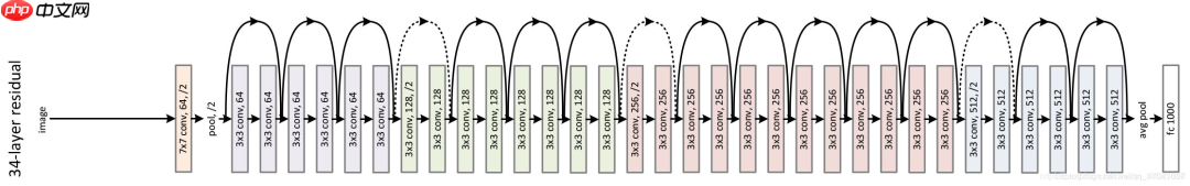
ResNet34的介绍 Kaiming He等人在2015年提出了ResNet,通过引入残差模块加深网络层数,在ImagNet数据集上的错误率降低到3.6%,超越了人眼识别水平。ResNet的设计思想深刻地影响了后来的深度神经网络的设计。
下图表示出了ResNet-34的结构。
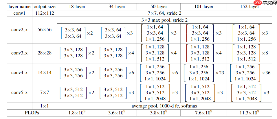
对比各版本的ResNet模型
- 使用飞桨高层API paddle.vision.models.resnet34() 直接调用图像分类resnet34网络
- ResNet34的实现和训练
#在./work/目录下有一个已经训练好的权重,若想使用已经训练好的权重,取消下行注释#!cp ./work/resnet34.pdparams ./
model = paddle.vision.models.resnet34(pretrained=True, num_classes = 7) #pretrained:表示是否加载在imagenet数据集上的预训练权重 num_classes由数据集的标签数决定lr = paddle.optimizer.lr.ReduceOnPlateau(learning_rate=0.0001, factor=0.5, patience=2, verbose=True)
opt = paddle.optimizer.Momentum(learning_rate=lr, momentum=0.9, parameters=model.parameters(), weight_decay=0.001) #选择momentum优化器# 启动训练过程train_pm(model, opt,loss_fct,EPOCH_NUM=30, model_name='resnet34')
- ResNet34的评估
use_gpu = Truepaddle.set_device('gpu:0') if use_gpu else paddle.set_device('cpu')
model = paddle.vision.models.resnet34(pretrained=True,num_classes = 7)
params_file_path = './resnet34.pdparams'model_state_dict = paddle.load(params_file_path)
model.load_dict(model_state_dict)#调用验证evaluation(model, loss_fct)
/opt/conda/envs/python35-paddle120-env/lib/python3.7/site-packages/paddle/fluid/dygraph/layers.py:1441: UserWarning: Skip loading for fc.weight. fc.weight receives a shape [512, 1000], but the expected shape is [512, 7].
  warnings.warn(("Skip loading for {}. ".format(key) + str(err)))
/opt/conda/envs/python35-paddle120-env/lib/python3.7/site-packages/paddle/fluid/dygraph/layers.py:1441: UserWarning: Skip loading for fc.bias. fc.bias receives a shape [1000], but the expected shape is [7].
  warnings.warn(("Skip loading for {}. ".format(key) + str(err)))
start evaluation .......
loss=0.9830, acc=0.6485
- 在使用resnet34进行300epoch训练后,准确率达到64.85%
- 在./work/目录下有一个已经训练好的ResNet34权重
9.2 学习率的设置
在深度学习神经网络模型中,通常使用标准的随机梯度下降算法更新参数,学习率代表参数更新幅度的大小,即步长。当学习率最优时,模型的有效容量最大,最终能达到的效果最好。学习率和深度学习任务类型有关,合适的学习率往往需要大量的实验和调参经验。探索学习率最优值时需要注意如下两点:
- 学习率不是越小越好。学习率越小,损失函数的变化速度越慢,意味着我们需要花费更长的时间进行收敛,如 图2 左图所示。
- 学习率不是越大越好。只根据总样本集中的一个批次计算梯度,抽样误差会导致计算出的梯度不是全局最优的方向,且存在波动。在接近最优解时,过大的学习率会导致参数在最优解附近震荡,损失难以收敛,如 图2 右图所示。
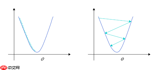
图2: 不同学习率(步长过大/过小)的示意图