本文围绕图像分割任务的EDA展开,以车道线检测为例构建通用模板。先介绍EDA重要性,接着统计图片像素信息,分析标签分布,包括含与不含背景类的情况,还探讨了标签均衡与不均衡的处理方法,最后进行重点图片分析及相关应用策略阐述。
☞☞☞AI 智能聊天, 问答助手, AI 智能搜索, 免费无限量使用 DeepSeek R1 模型☜☜☜

在完成目标检测任务的EDA模板开发后,本文继续探索图像分割任务的EDA。
什么是EDA?就是Exploratory Data Analysis,探索性数据分析。我们说工欲善其事,必先利其器;又说磨刀不误砍柴工,在算法模型开发的最佳实践中,EDA是必须的第一步。
在本文中,我们选取了最典型的图像分割场景之一——车道线检测任务,对数据集进行分析,以期形成一个较为通用的图像分割EDA模板。
# 解压数据集!unzip -oq /home/aistudio/data/data68698/智能车数据集.zip -d /home/aistudio/data
%cd data
/home/aistudio/data
%run make_list.py
[('image_4000/869.png', 'mask_4000/869.png'), ('image_4000/106.png', 'mask_4000/106.png'), ('image_4000/390.png', 'mask_4000/390.png')]
4000import osimport cv2import numpy as npfrom tqdm import tqdmimport matplotlib.pyplot as pltimport osfrom collections import Counterimport pandas as pdfrom pandas.core.frame import DataFramefrom PIL import Imageimport random %matplotlib inline
在图像分割任务中,数据集组织形式通常较为简单,一般就是有两个文件名一一对应的目录,比如标注文件长这样
images/xxx1.jpg (xx1.png) annotations/xxx1.png
images/xxx2.jpg (xx2.png) annotations/xxx2.png
……
然后标签文件labels.txt 每一行为一个单独的类别,相应的行号即为类别对应的id(行号从0开始),如下所示
labelA
labelB
……
图像分割任务本质上是对每个像素点的分布,因此,我们先统计下图片的像素标签分布信息。
#amount of classerCLASSES_NUM = 15#find image in folder dirdef findImages(dir,topdown=True):
    im_list = []    if not os.path.exists(dir):        print("Path for {} not exist!".format(dir))        raise
    else:        for root, dirs, files in os.walk(dir, topdown):            for fl in files:
                im_list.append(fl)    return im_list# 每一类别所包含的图像数量images_count = [0]*CLASSES_NUM# 每一类别的像素数目class_pixels_count = [0]*CLASSES_NUM# 每一类别对应的图像的总像素数目image_pixels_count = [0]*CLASSES_NUM

image_folder = './mask_4000'im_list = findImages(image_folder)

# 创建一个统计全部图片像素标签信息的DataFramesum_df = pd.DataFrame()for im in tqdm(im_list):    # 读取文件名
    # print(im)
    # 加载图片
    cv_img = cv2.imread(os.path.join(image_folder, im), cv2.IMREAD_UNCHANGED)
    size_img = cv_img.shape
    colors = set([])
    agg = []    for i in range(size_img[0]):        for j in range(size_img[1]):            # (i,j)位置像素点label
            p_value = cv_img.item(i,j)            # 检查像素点类别数是否正确
            if not p_value < CLASSES_NUM: # check
                print(p_value)            else:                # 给指定类别计数+1
                class_pixels_count[p_value] = class_pixels_count[p_value] + 1
                # 把像素点塞到set集合里
                colors.add(p_value)                # print(p_value)
                agg.append(p_value)
    im_size = size_img[0]*size_img[1]
    df = pd.DataFrame.from_dict(Counter(agg), orient='index')
    df = df.T
    df['filename'] = im
    df['sum_pixels'] = im_size    # print(df)
sum_df = sum_df.append(df, ignore_index=True)sum_df = sum_df.fillna(0)
# 分析列重排序column_names = ['filename', 'sum_pixels']
classes = [i for i in range(CLASSES_NUM)]
column_names.extend(classes)
sum_df = sum_df.loc[:,column_names]
# 生成各类别目标占比数据for i in range(CLASSES_NUM):
sum_df[str(i) + '_ratio'] = sum_df[i] / sum_df['sum_pixels']sum_df.head()
   filename  sum_pixels        0       1        2    3        4       5  \
0   869.png     2359296  2306267     0.0  10681.0  0.0  31493.0     0.0
1   106.png     2359296  2352657     0.0      0.0  0.0      0.0     0.0
2   390.png     2359296  2350482     0.0      0.0  0.0      0.0  8814.0
3  2256.png     2359296  2315716  2662.0   9939.0  0.0      0.0  3393.0
4  2968.png     2359296  2333629     0.0  10109.0  0.0  15558.0     0.0

         6    7  ...   5_ratio   6_ratio  7_ratio  8_ratio  9_ratio  10_ratio  \
0  10855.0  0.0  ...  0.000000  0.004601      0.0      0.0      0.0       0.0
1   6639.0  0.0  ...  0.000000  0.002814      0.0      0.0      0.0       0.0
2      0.0  0.0  ...  0.003736  0.000000      0.0      0.0      0.0       0.0
3  10854.0  0.0  ...  0.001438  0.004601      0.0      0.0      0.0       0.0
4      0.0  0.0  ...  0.000000  0.000000      0.0      0.0      0.0       0.0

   11_ratio  12_ratio  13_ratio  14_ratio
0  0.000000       0.0       0.0       0.0
1  0.000000       0.0       0.0       0.0
2  0.000000       0.0       0.0       0.0
3  0.007092       0.0       0.0       0.0
4  0.000000       0.0       0.0       0.0

[5 rows x 32 columns]# 保存分析数据sum_df.to_csv('../sum_df.csv', sep=',', header=True, index=True)a = sum_df.loc[:,classes].apply(lambda x:x.sum(),axis=0)
plt.figure(figsize=(12,12)) #调节图形大小labels = [str(i) for i in range(CLASSES_NUM)] #定义标签patches,text1,text2 = plt.pie(a,
                      labels=labels,
                      autopct = '%3.2f%%', #数值保留固定小数位
                      shadow = False, #无阴影设置
                      startangle =90, #逆时针起始角度设置
                      pctdistance = 0.6) #数值距圆心半径倍数距离#patches饼图的返回值,texts1饼图外label的文本,texts2饼图内部的文本# x,y轴刻度设置一致,保证饼图为圆形plt.axis('equal')
plt.show()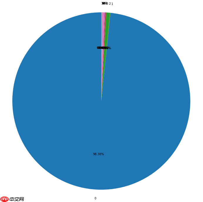
mask_pt = '/home/aistudio/data/mask_4000'count =  [0 for _ in range(16)]for m in tqdm(os.listdir(mask_pt)):
    pt = os.path.join(mask_pt, m)
    mask = cv2.imread(pt, 0)
    size = mask.shape[0] * mask.shape[1]    for i in range(16):
        a = mask == i
        ratio_i = np.sum(a.astype(np.float)) / size
        count[i] += ratio_i

sum_ = np.sum(count[1:])
ratios = [v/sum_ for v in count[1:]]for i in range(0, len(ratios)): print('-[INFO] Label {}: {:.4f}'.format(i+1, ratios[i]))-[INFO] Label 1: 0.0170 -[INFO] Label 2: 0.4482 -[INFO] Label 3: 0.0843 -[INFO] Label 4: 0.0767 -[INFO] Label 5: 0.0334 -[INFO] Label 6: 0.2513 -[INFO] Label 7: 0.0070 -[INFO] Label 8: 0.0025 -[INFO] Label 9: 0.0158 -[INFO] Label 10: 0.0152 -[INFO] Label 11: 0.0292 -[INFO] Label 12: 0.0087 -[INFO] Label 13: 0.0061 -[INFO] Label 14: 0.0046 -[INFO] Label 15: 0.0000
plt.figure(figsize=(24,24)) #调节图形大小labels = [str(i) for i in range(1, 16)] #定义标签patches,text1,text2 = plt.pie(ratios,
                      labels=labels,
                      autopct = '%3.2f%%', #数值保留固定小数位
                      shadow = False, #无阴影设置
                      startangle =90, #逆时针起始角度设置
                      pctdistance = 0.6) #数值距圆心半径倍数距离#patches饼图的返回值,texts1饼图外label的文本,texts2饼图内部的文本# x,y轴刻度设置一致,保证饼图为圆形plt.axis('equal')
plt.show()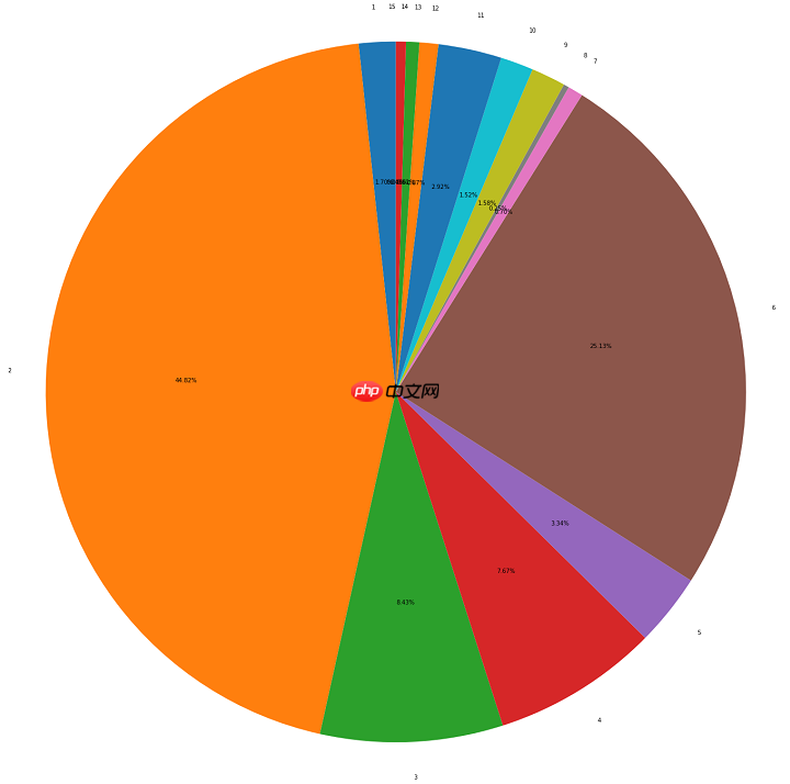
分析标签分布情况,是做好图像分割模型开发的先决条件。
显然,这会是我们比较希望看到的情况。如果标签均衡分布,可以考虑直接开始训练了。如果觉得样本量不是很够,还可以加入数据增强策略。
比如在PaddleSeg中,就给出了下列数据增强策略 在PaddleSeg的config文件里进行修改。
| Resize方式 | 配置参数 | 含义 | 备注 |
|---|---|---|---|
| Unpadding | AUG.FIX_RESIZE_SIZE | Resize的固定尺寸 | |
| Step-Scaling | AUG.MIN_SCALE_FACTOR | Resize最小比例 | |
| AUG.MAX_SCALE_FACTOR | Resize最大比例 | ||
| AUG.SCALE_STEP_SIZE | Resize比例选取的步长 | ||
| Range-Scaling | AUG.MIN_RESIZE_VALUE | 图像长边变动范围的最小值 | |
| AUG.MAX_RESIZE_VALUE | 图像长边变动范围的最大值 | ||
| AUG.INF_RESIZE_VALUE | 预测时长边对齐时所指定的固定长度 | 取值必须在 | |
| [AUG.MIN_RESIZE_VALUE, | |||
| AUG.MAX_RESIZE_VALUE] | |||
| 范围内。 |
很不幸,在真实应用场景中,标签分布不均衡才是常态。这时主要的处理方法可以考虑:
在这里,数据增强是对某类别标签的单独增强,可以考虑离线构建补充的增强数据,从而是新的数据集回到整体的平衡态中。
而Loss优化方面,可以考虑以Lovasz loss为代表的损失函数设置。
Lovasz loss基于子模损失(submodular losses)的凸Lovasz扩展,对神经网络的mean IoU损失进行优化。Lovasz loss根据分割目标的类别数量可分为两种:lovasz hinge loss和lovasz softmax loss. 其中lovasz hinge loss适用于二分类问题,lovasz softmax loss适用于多分类问题。相关论文可参考参考文献查看具体原理。
在PaddleSeg中,推荐以下两种训练方式

抖猫高清去水印微信小程序,源码为短视频去水印微信小程序全套源码,包含微信小程序端源码,服务端后台源码,支持某音、某手、某书、某站短视频平台去水印,提供全套的源码,实现功能包括:1、小程序登录授权、获取微信头像、获取微信用户2、首页包括:流量主已经对接、去水印连接解析、去水印操作指导、常见问题指引3、常用工具箱:包括视频镜头分割(可自定义时长分割)、智能分割(根据镜头自动分割)、视频混剪、模糊图片高
 0
0

更详细的介绍可参考链接
一般的分割库使用单通道灰度图作为标注图片,往往显示出来是全黑的效果。灰度标注图在可视化的时候效果不佳。
PaddleSeg支持伪彩色图作为标注图片,在原来的单通道图片基础上,注入调色板。在基本不增加图片大小的基础上,却可以显示出彩色的效果。
本文使用的就是PaddleSeg提供的转换脚本gray2pseudo_color.py。
image_pt = '/home/aistudio/data/image_4000/'pseudo_color_pt = '/home/aistudio/data/color_4000/'
!mkdir color_4000
!python ../gray2pseudo_color.py mask_4000 color_4000
def plot_image_examples(df, rows=3, cols=3, title='Image examples'):
    fig, axs = plt.subplots(rows, cols, figsize=(16,16))    if title=='Image examples':        for row in range(rows):            for col in range(cols):
                idx = np.random.randint(len(df), size=1)[0]
                name = df.iloc[idx]["filename"]
                img = Image.open(image_pt + str(name))
                axs[row, col].imshow(img)
                axs[row, col].axis('off')    else:        for row in range(rows):            for col in range(cols):
                idx = np.random.randint(len(df), size=1)[0]
                name = df.iloc[idx]["filename"]
                img = Image.open(pseudo_color_pt + str(name))
                axs[row, col].imshow(img)
                axs[row, col].axis('off')
plt.suptitle(title)sum_df = pd.read_csv('../sum_df.csv',index_col='Unnamed: 0')sum_df.head()
   filename  sum_pixels        0       1        2    3        4       5  \
0   869.png     2359296  2306267     0.0  10681.0  0.0  31493.0     0.0
1   106.png     2359296  2352657     0.0      0.0  0.0      0.0     0.0
2   390.png     2359296  2350482     0.0      0.0  0.0      0.0  8814.0
3  2256.png     2359296  2315716  2662.0   9939.0  0.0      0.0  3393.0
4  2968.png     2359296  2333629     0.0  10109.0  0.0  15558.0     0.0

         6    7  ...   5_ratio   6_ratio  7_ratio  8_ratio  9_ratio  10_ratio  \
0  10855.0  0.0  ...  0.000000  0.004601      0.0      0.0      0.0       0.0
1   6639.0  0.0  ...  0.000000  0.002814      0.0      0.0      0.0       0.0
2      0.0  0.0  ...  0.003736  0.000000      0.0      0.0      0.0       0.0
3  10854.0  0.0  ...  0.001438  0.004601      0.0      0.0      0.0       0.0
4      0.0  0.0  ...  0.000000  0.000000      0.0      0.0      0.0       0.0

   11_ratio  12_ratio  13_ratio  14_ratio
0  0.000000       0.0       0.0       0.0
1  0.000000       0.0       0.0       0.0
2  0.000000       0.0       0.0       0.0
3  0.007092       0.0       0.0       0.0
4  0.000000       0.0       0.0       0.0

[5 rows x 32 columns]以类别1为例,展示像素点少于500个的原图和标注图片。
less_spikes_ids = sum_df[sum_df['1']>0][sum_df['1']<500].sort_values(by='1',ascending=False).filename
plot_image_examples(sum_df[sum_df.filename.isin(less_spikes_ids)])
/opt/conda/envs/python35-paddle120-env/lib/python3.7/site-packages/ipykernel_launcher.py:1: UserWarning: Boolean Series key will be reindexed to match DataFrame index.
  """Entry point for launching an IPython kernel.
<Figure size 1152x1152 with 9 Axes>
plot_image_examples(sum_df[sum_df.filename.isin(less_spikes_ids)],title='Mask examples')
<Figure size 1152x1152 with 9 Axes>
less_spikes_ids = sum_df[sum_df['2']>0][sum_df['2']<500].sort_values(by='2',ascending=False).filename
plot_image_examples(sum_df[sum_df.filename.isin(less_spikes_ids)])
plot_image_examples(sum_df[sum_df.filename.isin(less_spikes_ids)],title='Mask examples')
/opt/conda/envs/python35-paddle120-env/lib/python3.7/site-packages/ipykernel_launcher.py:1: UserWarning: Boolean Series key will be reindexed to match DataFrame index.
  """Entry point for launching an IPython kernel.
<Figure size 1152x1152 with 9 Axes>
<Figure size 1152x1152 with 9 Axes>
以类别1为例,展示大目标的原图和标注图片。
less_spikes_ids = sum_df[sum_df['1']>max(sum_df['1'])*0.9].sort_values(by='1',ascending=False).filename
plot_image_examples(sum_df[sum_df.filename.isin(less_spikes_ids)])
plot_image_examples(sum_df[sum_df.filename.isin(less_spikes_ids)],title='Mask examples')
<Figure size 1152x1152 with 9 Axes>
<Figure size 1152x1152 with 9 Axes>
less_spikes_ids = sum_df[sum_df['2']>max(sum_df['2'])*0.9].sort_values(by='2',ascending=False).filename
plot_image_examples(sum_df[sum_df.filename.isin(less_spikes_ids)])
plot_image_examples(sum_df[sum_df.filename.isin(less_spikes_ids)],title='Mask examples')
<Figure size 1152x1152 with 9 Axes>
<Figure size 1152x1152 with 9 Axes>
以类别1、2、3为例,随机展示三者并存时的原图和标注图片。
sum_df[sum_df['1']>0][sum_df['2']>0][sum_df['3']>0].sort_values(by=str(i),ascending=False).filename
plot_image_examples(sum_df[sum_df.filename.isin(less_spikes_ids)])
plot_image_examples(sum_df[sum_df.filename.isin(less_spikes_ids)],title='Mask examples')
/opt/conda/envs/python35-paddle120-env/lib/python3.7/site-packages/ipykernel_launcher.py:1: UserWarning: Boolean Series key will be reindexed to match DataFrame index.
  """Entry point for launching an IPython kernel.
/opt/conda/envs/python35-paddle120-env/lib/python3.7/site-packages/ipykernel_launcher.py:1: UserWarning: Boolean Series key will be reindexed to match DataFrame index.
  """Entry point for launching an IPython kernel.
<Figure size 1152x1152 with 9 Axes>
<Figure size 1152x1152 with 9 Axes>
重点图片分析首先再次印证了图像分割数据集的标签分布情况,而对于标签分布不均衡问题,处理方式在章节2.2中做了详细说明。
同时,在重点图片分析过程中,我们也可以确认,数据集中是否存在会影响模型精度的困难样本,并针对性地予以解决。
具体策略上,依然与Loss的选择密切相关。这里的重点是引入了OHEM,OHEM旨在解决处理困难样本的问题。OHEM算法将根据输入到模型中的样本的损失来区分出困难样本,这些困难样本分类精度差,会产生较大的损失。
class paddleseg.models.losses.OhemCrossEntropyLoss(
                thresh = 0.7,
                min_kept = 10000,
                ignore_index = 255
)如果还需要提高边缘检测效果,可用:
OhemEdgeAttentionLoss
class paddleseg.models.losses.OhemEdgeAttentionLoss(
                edge_threshold = 0.8,
                thresh = 0.7,
                min_kept = 5000,
                ignore_index = 255
)以上就是图像语义分割EDA模板的详细内容,更多请关注php中文网其它相关文章!

每个人都需要一台速度更快、更稳定的 PC。随着时间的推移,垃圾文件、旧注册表数据和不必要的后台进程会占用资源并降低性能。幸运的是,许多工具可以让 Windows 保持平稳运行。

 广告
广告Copyright 2014-2025 https://www.php.cn/ All Rights Reserved | php.cn | 湘ICP备2023035733号


 709
709