该内容围绕二手车交易价格预测大赛展开,介绍赛题是回归问题,需根据给定数据集预测价格。说明了数据来源、训练集和测试集划分,以及各变量信息。还涵盖数据读取、探索、分析,模型训练(如xgb、lgb)、预测、融合等流程,包括特征工程和模型优化等内容。
☞☞☞AI 智能聊天, 问答助手, AI 智能搜索, 免费无限量使用 DeepSeek R1 模型☜☜☜

二手车交易价格预测大赛赛题以二手车市场为背景,要求选手预测二手汽车的交易价格,这是一个是非常经典项目的回归问题。为了更好的引导大家入门,本项目设置了系列学习方案,其中包括数据科学库、通用流程和baseline方案学习三部分。通过对本方案的完整学习,可以帮助掌握数据竞赛基本技能。现让更多对机器学习感兴趣小伙伴可以上手实战一下,因篇幅内容限制,将原学习项目拆解成多个notebook方便学习,只需一键fork。
推荐项目:【机器学习入门与实践】合集入门必看系列,含数据挖掘项目实战
方便入门同学快速掌握相关知识进行实战
比赛要求参赛选手根据给定的数据集,建立模型,二手汽车的交易价格。
来自 Ebay Kleinanzeigen 报废的二手车,数量超过 370,000,包含 20 列变量信息,为了保证 比赛的公平性,将会从中抽取 10 万条作为训练集,5 万条作为测试集 A,5 万条作为测试集 B。同时会对名称、车辆类型、变速箱、model、燃油类型、品牌、公里数、价格等信息进行 脱敏。
一般而言,对于数据在比赛界面都有对应的数据概况介绍(匿名特征除外),说明列的性质特征。了解列的性质会有助于我们对于数据的理解和后续分析。 Tip:匿名特征,就是未告知数据列所属的性质的特征列。
train.csv
数字全都脱敏处理,都为label encoding形式,即数字形式
本赛题的评价标准为MAE(Mean Absolute Error):
MAE=n∑i=1n∣yi−y^i∣
其中yi代表第i个样本的真实值,其中y^i代表第i个样本的预测值。
一般问题评价指标说明:
什么是评估指标:
评估指标即是我们对于一个模型效果的数值型量化。(有点类似与对于一个商品评价打分,而这是针对于模型效果和理想效果之间的一个打分)
一般来说分类和回归问题的评价指标有如下一些形式:
分类算法常见的评估指标如下:
对于回归预测类常见的评估指标如下:
平均绝对误差 平均绝对误差(Mean Absolute Error,MAE):平均绝对误差,其能更好地反映预测值与真实值误差的实际情况,其计算公式如下:
MAE=N1i=1∑N∣yi−y^i∣
均方误差 均方误差(Mean Squared Error,MSE),均方误差,其计算公式为:
MSE=N1i=1∑N(yi−y^i)2
R2(R-Square)的公式为: 残差平方和:
SSres=∑(yi−y^i)2
总平均值:
SStot=∑(yi−yi)2
其中y表示y的平均值 得到R2表达式为:
R2=1−SStotSSres=1−∑(yi−y)2∑(yi−y^i)2
R2用于度量因变量的变异中可由自变量解释部分所占的比例,取值范围是 0~1,R2越接近1,表明回归平方和占总平方和的比例越大,回归线与各观测点越接近,用x的变化来解释y值变化的部分就越多,回归的拟合程度就越好。所以R2也称为拟合优度(Goodness of Fit)的统计量。
yi表示真实值,y^i表示预测值,yi表示样本均值。得分越高拟合效果越好。
了解赛题
赛题概况
数据概况
预测指标
分析赛题
数据读取pandas
分类指标评价计算示例
回归指标评价计算示例
EDA探索
特征工程
建模调参,相关原理介绍与推荐
模型融合
# 下载数据!wget http://tianchi-media.oss-cn-beijing.aliyuncs.com/dragonball/DM/data.zip# 解压下载好的数据!unzip data.zip
# 导入函数工具## 基础工具import numpy as npimport pandas as pdimport warningsimport matplotlibimport matplotlib.pyplot as pltimport seaborn as snsfrom scipy.special import jnfrom IPython.display import display, clear_outputimport time

warnings.filterwarnings('ignore')
%matplotlib inline## 模型预测的from sklearn import linear_modelfrom sklearn import preprocessingfrom sklearn.svm import SVRfrom sklearn.ensemble import RandomForestRegressor,GradientBoostingRegressor## 数据降维处理的from sklearn.decomposition import PCA,FastICA,FactorAnalysis,SparsePCAimport lightgbm as lgbimport xgboost as xgb## 参数搜索和评价的from sklearn.model_selection import GridSearchCV,cross_val_score,StratifiedKFold,train_test_splitfrom sklearn.metrics import mean_squared_error, mean_absolute_error## 通过Pandas对于数据进行读取 (pandas是一个很友好的数据读取函数库)Train_data = pd.read_csv('/home/aistudio/dataset/used_car_train_20200313.csv', sep=' ')
TestA_data = pd.read_csv('/home/aistudio/dataset/used_car_testA_20200313.csv', sep=' ')## 输出数据的大小信息print('Train data shape:',Train_data.shape)print('TestA data shape:',TestA_data.shape)Train data shape: (150000, 31) TestA data shape: (50000, 30)
## 通过.head() 简要浏览读取数据的形式Train_data.head()
   SaleID    name   regDate  model  brand  bodyType  fuelType  gearbox  power  \
0       0     736  20040402   30.0      6       1.0       0.0      0.0     60
1       1    2262  20030301   40.0      1       2.0       0.0      0.0      0
2       2   14874  20040403  115.0     15       1.0       0.0      0.0    163
3       3   71865  19960908  109.0     10       0.0       0.0      1.0    193
4       4  111080  20120103  110.0      5       1.0       0.0      0.0     68

   kilometer  ...       v_5       v_6       v_7       v_8       v_9      v_10  \
0       12.5  ...  0.235676  0.101988  0.129549  0.022816  0.097462 -2.881803
1       15.0  ...  0.264777  0.121004  0.135731  0.026597  0.020582 -4.900482
2       12.5  ...  0.251410  0.114912  0.165147  0.062173  0.027075 -4.846749
3       15.0  ...  0.274293  0.110300  0.121964  0.033395  0.000000 -4.509599
4        5.0  ...  0.228036  0.073205  0.091880  0.078819  0.121534 -1.896240

       v_11      v_12      v_13      v_14
0  2.804097 -2.420821  0.795292  0.914762
1  2.096338 -1.030483 -1.722674  0.245522
2  1.803559  1.565330 -0.832687 -0.229963
3  1.285940 -0.501868 -2.438353 -0.478699
4  0.910783  0.931110  2.834518  1.923482

[5 rows x 31 columns]## 通过 .info() 简要可以看到对应一些数据列名,以及NAN缺失信息Train_data.info()
<class 'pandas.core.frame.DataFrame'>
RangeIndex: 150000 entries, 0 to 149999
Data columns (total 31 columns):
 #   Column             Non-Null Count   Dtype
---  ------             --------------   -----
 0   SaleID             150000 non-null  int64
 1   name               150000 non-null  int64
 2   regDate            150000 non-null  int64
 3   model              149999 non-null  float64
 4   brand              150000 non-null  int64
 5   bodyType           145494 non-null  float64
 6   fuelType           141320 non-null  float64
 7   gearbox            144019 non-null  float64
 8   power              150000 non-null  int64
 9   kilometer          150000 non-null  float64
 10  notRepairedDamage  150000 non-null  object
 11  regionCode         150000 non-null  int64
 12  seller             150000 non-null  int64
 13  offerType          150000 non-null  int64
 14  creatDate          150000 non-null  int64
 15  price              150000 non-null  int64
 16  v_0                150000 non-null  float64
 17  v_1                150000 non-null  float64
 18  v_2                150000 non-null  float64
 19  v_3                150000 non-null  float64
 20  v_4                150000 non-null  float64
 21  v_5                150000 non-null  float64
 22  v_6                150000 non-null  float64
 23  v_7                150000 non-null  float64
 24  v_8                150000 non-null  float64
 25  v_9                150000 non-null  float64
 26  v_10               150000 non-null  float64
 27  v_11               150000 non-null  float64
 28  v_12               150000 non-null  float64
 29  v_13               150000 non-null  float64
 30  v_14               150000 non-null  float64
dtypes: float64(20), int64(10), object(1)
memory usage: 35.5+ MB
## 通过 .columns 查看列名Train_data.columns
Index(['SaleID', 'name', 'regDate', 'model', 'brand', 'bodyType', 'fuelType',
       'gearbox', 'power', 'kilometer', 'notRepairedDamage', 'regionCode',
       'seller', 'offerType', 'creatDate', 'price', 'v_0', 'v_1', 'v_2', 'v_3',
       'v_4', 'v_5', 'v_6', 'v_7', 'v_8', 'v_9', 'v_10', 'v_11', 'v_12',
       'v_13', 'v_14'],
dtype='object')TestA_data.info()
<class 'pandas.core.frame.DataFrame'>
RangeIndex: 50000 entries, 0 to 49999
Data columns (total 30 columns):
 #   Column             Non-Null Count  Dtype
---  ------             --------------  -----
 0   SaleID             50000 non-null  int64
 1   name               50000 non-null  int64
 2   regDate            50000 non-null  int64
 3   model              50000 non-null  float64
 4   brand              50000 non-null  int64
 5   bodyType           48587 non-null  float64
 6   fuelType           47107 non-null  float64
 7   gearbox            48090 non-null  float64
 8   power              50000 non-null  int64
 9   kilometer          50000 non-null  float64
 10  notRepairedDamage  50000 non-null  object
 11  regionCode         50000 non-null  int64
 12  seller             50000 non-null  int64
 13  offerType          50000 non-null  int64
 14  creatDate          50000 non-null  int64
 15  v_0                50000 non-null  float64
 16  v_1                50000 non-null  float64
 17  v_2                50000 non-null  float64
 18  v_3                50000 non-null  float64
 19  v_4                50000 non-null  float64
 20  v_5                50000 non-null  float64
 21  v_6                50000 non-null  float64
 22  v_7                50000 non-null  float64
 23  v_8                50000 non-null  float64
 24  v_9                50000 non-null  float64
 25  v_10               50000 non-null  float64
 26  v_11               50000 non-null  float64
 27  v_12               50000 non-null  float64
 28  v_13               50000 non-null  float64
 29  v_14               50000 non-null  float64
dtypes: float64(20), int64(9), object(1)
memory usage: 11.4+ MB
## 通过 .describe() 可以查看数值特征列的一些统计信息Train_data.describe()
              SaleID           name       regDate          model  \
count  150000.000000  150000.000000  1.500000e+05  149999.000000
mean    74999.500000   68349.172873  2.003417e+07      47.129021
std     43301.414527   61103.875095  5.364988e+04      49.536040
min         0.000000       0.000000  1.991000e+07       0.000000
25%     37499.750000   11156.000000  1.999091e+07      10.000000
50%     74999.500000   51638.000000  2.003091e+07      30.000000
75%    112412499.250000  118841.250000  2.007111e+07      66.000000
max    149999.000000  196812.000000  2.015121e+07     247.000000

               brand       bodyType       fuelType        gearbox  \
count  150000.000000  145494.000000  141320.000000  144019.000000
mean        8.052733       1.792369       0.375842       0.224943
std         7.864956       1.760640       0.548677       0.417546
min         0.000000       0.000000       0.000000       0.000000
25%         1.000000       0.000000       0.000000       0.000000
50%         6.000000       1.000000       0.000000       0.000000
75%        13.000000       3.000000       1.000000       0.000000
max        39.000000       7.000000       6.000000       1.000000

               power      kilometer  ...            v_5            v_6  \
count  150000.000000  150000.000000  ...  150000.000000  150000.000000
mean      119.316547      12.597160  ...       0.248204       0.044923
std       177.168419       3.919576  ...       0.045804       0.051743
min         0.000000       0.500000  ...       0.000000       0.000000
25%        75.000000      12.500000  ...       0.243615       0.000038
50%       110.000000      15.000000  ...       0.257798       0.000812
75%       150.000000      15.000000  ...       0.265297       0.102009
max     19312.000000      15.000000  ...       0.291838       0.151420

                 v_7            v_8            v_9           v_10  \
count  150000.000000  150000.000000  150000.000000  150000.000000
mean        0.124124692       0.058144       0.061996      -0.001000
std         0.201410       0.029186       0.035692       3.772386
min         0.000000       0.000000       0.000000      -9.168192
25%         0.062474       0.035334       0.033930      -3.722303
50%         0.095866       0.057014       0.058484       1.624076
75%         0.125243       0.079382       0.087491       2.844357
max         1.404936       0.160791       0.222787      12.357011

                v_11           v_12           v_13           v_14
count  150000.000000  150000.000000  150000.000000  150000.000000
mean        0.009035       0.004813       0.000313      -0.000688
std         3.286071       2.517478       1.288988       1.038685
min        -5.558207      -9.639552      -4.153899      -6.546556
25%        -1.951543      -1.871846      -1.057789      -0.437034
50%        -0.358053      -0.130753      -0.036245       0.141241246
75%         1.255022       1.776933       0.942813       0.680378
max        18.819042      13.847792      11.147669       8.658418

[8 rows x 30 columns]TestA_data.describe()
              SaleID           name       regDate         model         brand  \
count   50000.000000   50000.000000  5.000000e+04  50000.000000  50000.000000
mean   174999.500000   68542.223280  2.003393e+07     46.844520      8.056240
std     14433.901067   61052.808133  5.368870e+04     49.469548      7.819477
min    150000.000000       0.000000  1.991000e+07      0.000000      0.000000
25%    162499.750000   11203.500000  1.999091e+07     10.000000      1.000000
50%    174999.500000   52248.500000  2.003091e+07     29.000000      6.000000
75%    187499.250000  118856.500000  2.007110e+07     65.000000     13.000000
max    199999.000000  196805.000000  2.015121e+07    246.000000     39.000000

           bodyType      fuelType       gearbox         power     kilometer  \
count  48587.000000  47107.000000  48090.000000  50000.000000  50000.000000
mean       1.782185      0.373405      0.224350    119.883620     12.595580
std        1.760736      0.546442      0.417158    185.097387      3.908979
min        0.000000      0.000000      0.000000      0.000000      0.500000
25%        0.000000      0.000000      0.000000     75.000000     12.500000
50%        1.000000      0.000000      0.000000    109.000000     15.000000
75%        3.000000      1.000000      0.000000    150.000000     15.000000
max        7.000000      6.000000      1.000000  20000.000000     15.000000

       ...           v_5           v_6           v_7           v_8  \
count  ...  50000.000000  50000.000000  50000.000000  50000.000000
mean   ...      0.248669      0.045021      0.122744      0.057997
std    ...      0.044601      0.051766      0.195972      0.029211
min    ...      0.000000      0.000000      0.000000      0.000000
25%    ...      0.243762      0.000044      0.062644      0.035084
50%    ...      0.257877      0.000815      0.095828      0.057084
75%    ...      0.265328      0.102025      0.125438      0.079077
max    ...      0.291618      0.153265      1.358813      0.156355

                v_9          v_10          v_11          v_12          v_13  \
count  50000.000000  50000.000000  50000.000000  50000.000000  50000.000000
mean       0.062000     -0.017855     -0.013742     -0.013554     -0.003147
std        0.035653      3.747985      3.231258      2.515962      1.286597
min        0.000000     -9.160049     -5.411964     -8.916949     -4.123333
25%        0.033714     -3.700121     -1.971325     -1.876703     -1.060428
50%        0.058764      1.613212     -0.355843     -0.142779     -0.035956
75%        0.087489      2.832708      1.262914      1.764335      0.941469
max        0.214775     12.338872     18.856218     12.950498      5.913273

               v_14
count  50000.000000
mean       0.001516
std        1.027360
min       -6.112667
25%       -0.437920
50%        0.138799
75%        0.681163
max        2.624622

[8 rows x 29 columns]#### 1) 提取数值类型特征列名numerical_cols = Train_data.select_dtypes(exclude = 'object').columnsprint(numerical_cols)
Index(['SaleID', 'name', 'regDate', 'model', 'brand', 'bodyType', 'fuelType',
       'gearbox', 'power', 'kilometer', 'regionCode', 'seller', 'offerType',
       'creatDate', 'price', 'v_0', 'v_1', 'v_2', 'v_3', 'v_4', 'v_5', 'v_6',
       'v_7', 'v_8', 'v_9', 'v_10', 'v_11', 'v_12', 'v_13', 'v_14'],
dtype='object')categorical_cols = Train_data.select_dtypes(include = 'object').columnsprint(categorical_cols)
Index(['notRepairedDamage'], dtype='object')
#### 2) 构建训练和测试样本## 选择特征列feature_cols = [col for col in numerical_cols if col not in ['SaleID','name','regDate','creatDate','price','model','brand','regionCode','seller']]
feature_cols = [col for col in feature_cols if 'Type' not in col]## 提前特征列,标签列构造训练样本和测试样本X_data = Train_data[feature_cols]
Y_data = Train_data['price']

X_test = TestA_data[feature_cols]print('X train shape:',X_data.shape)print('X test shape:',X_test.shape)X train shape: (150000, 18) X test shape: (50000, 18)
## 定义了一个统计函数,方便后续信息统计def Sta_inf(data):
print('_min',np.min(data)) print('_max:',np.max(data)) print('_mean',np.mean(data)) print('_ptp',np.ptp(data)) print('_std',np.std(data)) print('_var',np.var(data))#### 3) 统计标签的基本分布信息print('Sta of label:')
Sta_inf(Y_data)Sta of label: _min 11 _max: 99999 _mean 5923.327333333334 _ptp 99988 _std 7501.973469876635 _var 56279605.942732885
## 绘制标签的统计图,查看标签分布plt.hist(Y_data)
plt.show()
plt.close()
<Figure size 640x480 with 1 Axes>
#### 4) 缺省值用-1填补X_data = X_data.fillna(-1)
X_test = X_test.fillna(-1)
## xgb-Modelxgr = xgb.XGBRegressor(n_estimators=120, learning_rate=0.1, gamma=0, subsample=0.8,\
        colsample_bytree=0.9, max_depth=7) #,objective ='reg:squarederror'scores_train = []
scores = []## 5折交叉验证方式sk=StratifiedKFold(n_splits=5,shuffle=True,random_state=0)for train_ind,val_ind in sk.split(X_data,Y_data):

    train_x=X_data.iloc[train_ind].values
    train_y=Y_data.iloc[train_ind]
    val_x=X_data.iloc[val_ind].values
    val_y=Y_data.iloc[val_ind]

    xgr.fit(train_x,train_y)
    pred_train_xgb=xgr.predict(train_x)
    pred_xgb=xgr.predict(val_x)

    score_train = mean_absolute_error(train_y,pred_train_xgb)
    scores_train.append(score_train)
    score = mean_absolute_error(val_y,pred_xgb)
scores.append(score)print('Train mae:',np.mean(score_train))print('Val mae',np.mean(scores))def build_model_xgb(x_train,y_train):
model = xgb.XGBRegressor(n_estimators=150, learning_rate=0.1, gamma=0, subsample=0.8,\
colsample_bytree=0.9, max_depth=7) #, objective ='reg:squarederror'
model.fit(x_train, y_train) return modeldef build_model_lgb(x_train,y_train):
estimator = lgb.LGBMRegressor(num_leaves=127,n_estimators = 150)
param_grid = { 'learning_rate': [0.01, 0.05, 0.1, 0.2],
}
gbm = GridSearchCV(estimator, param_grid)
gbm.fit(x_train, y_train) return gbm## Split data with valx_train,x_val,y_train,y_val = train_test_split(X_data,Y_data,test_size=0.3)
print('Train lgb...')
model_lgb = build_model_lgb(x_train,y_train)
val_lgb = model_lgb.predict(x_val)
MAE_lgb = mean_absolute_error(y_val,val_lgb)print('MAE of val with lgb:',MAE_lgb)print('Predict lgb...')
model_lgb_pre = build_model_lgb(X_data,Y_data)
subA_lgb = model_lgb_pre.predict(X_test)print('Sta of Predict lgb:')
Sta_inf(subA_lgb)print('Train xgb...')
model_xgb = build_model_xgb(x_train,y_train)
val_xgb = model_xgb.predict(x_val)
MAE_xgb = mean_absolute_error(y_val,val_xgb)print('MAE of val with xgb:',MAE_xgb)print('Predict xgb...')
model_xgb_pre = build_model_xgb(X_data,Y_data)
subA_xgb = model_xgb_pre.predict(X_test)print('Sta of Predict xgb:')
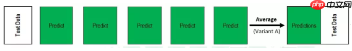
Sta_inf(subA_xgb)## 这里我们采取了简单的加权融合的方式val_Weighted = (1-MAE_lgb/(MAE_xgb+MAE_lgb))*val_lgb+(1-MAE_xgb/(MAE_xgb+MAE_lgb))*val_xgb
val_Weighted[val_Weighted<0]=10 # 由于我们发现预测的最小值有负数,而真实情况下,price为负是不存在的,由此我们进行对应的后修正print('MAE of val with Weighted ensemble:',mean_absolute_error(y_val,val_Weighted))sub_Weighted = (1-MAE_lgb/(MAE_xgb+MAE_lgb))*subA_lgb+(1-MAE_xgb/(MAE_xgb+MAE_lgb))*subA_xgb## 查看预测值的统计进行plt.hist(Y_data) plt.show() plt.close()
sub = pd.DataFrame()
sub['SaleID'] = TestA_data.SaleID
sub['price'] = sub_Weighted
sub.to_csv('./sub_Weighted.csv',index=False)sub.head()
因篇幅内容限制,将原学习项目拆解成多个notebook方便学习,只需一键fork。

简单加权融合:
stacking/blending:
boosting/bagging(在xgboost,Adaboost,GBDT中已经用到):
训练:
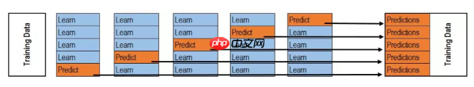
预测:
以上就是【机器学习入门与实践】二手车价格交易预测含EDA、特征工程、特征优化、模型融合的详细内容,更多请关注php中文网其它相关文章!

每个人都需要一台速度更快、更稳定的 PC。随着时间的推移,垃圾文件、旧注册表数据和不必要的后台进程会占用资源并降低性能。幸运的是,许多工具可以让 Windows 保持平稳运行。

 广告
广告Copyright 2014-2025 https://www.php.cn/ All Rights Reserved | php.cn | 湘ICP备2023035733号


 280
280