『行远见大』PaddlePaddle2.0 使用教学-人工智能-PHP中文网

本文为PaddlePaddle2.0使用教学，涵盖张量与numpy数组转换、操作及维度调整，自动微分、计算图、CUDA语义等基础，还介绍神经网络模块（线性层、激活函数等）、损失函数（MSE、交叉熵）、优化器（SGD、Momentum）及学习率调度器，附线性回归和神经网络拟合数据实例。

☞☞☞AI 智能聊天, 问答助手, AI 智能搜索, 免费无限量使用 DeepSeek R1 模型☜☜☜

『行远见大』paddlepaddle2.0 使用教学 - php中文网

行远见大』PaddlePaddle2.0 使用教学

本项目同时也是李宏毅机器学习课后作业”Paddle2.0基础练习“。

向开源致敬！

大家好，我是行远见大。这里有我学习机器学习的笔记与心得。欢迎你与我一同建设飞桨开源社区，知识分享是一种美德，让我们向开源致敬！

PaddlePaddle教学

项目描述

此教程旨在介绍PaddlePaddle(一个易用、高效、灵活、可扩展的深度学习框架)，根据PaddlePaddle 2.0 rc官方手册编写，介绍了PaddlePaddle中比较常用的一些API以及其基本用法。

数据集介绍

无

项目要求

学会使用自动微分（一个强大的实用工具）
使用PaddlePaddle实现深度学习中的常用功能
使用paddle.io.Dataset处理数据
了解PaddlePaddle中的自动混合精度训练

数据准备

无

环境配置/安装

无

PaddlePaddle 介绍

此教程根据 PaddlePaddle 2.0 rc官方手册编写。

此教程旨在介绍PaddlePaddle(一个易用、高效、灵活、可扩展的深度学习框架)
本教程只介绍了paddle中比较常用的一些API以及其基本用法，并不全面，如有任何问题请参考PaddlePaddle 2.0 rc官方手册，也可以百度一下

你将收获以下知识：

自动微分是一个强大的实用工具
使用PaddlePaddle实现深度学习中的常用函数
使用paddle.io.Dataset处理数据
PaddlePaddle中的自动混合精度训练

Paddle中张量以及张量和numpy数组之间的转换

到目前为止，我们已经使用了不少和numpy数组相关的操作。作为PaddlePaddle中数据处理的基本元素，张量tensor和numpy数组中的ndarray非常相似。

In [1]

import paddleimport paddle.fluid as fluidimport numpy as np
paddle.disable_static()# 使用创建numpy数组相同的方式来创建Tensorx_numpy = np.array([[2.5, 2.5], [2.5, 2.5], [2.5, 2.5]])
x_paddle = paddle.to_tensor(x_numpy)# [[2.5, 2.5], [2.5, 2.5], [2.5, 2.5]]data = fluid.layers.fill_constant(shape=[3, 2], value=2.5, dtype='float64')
x_paddle = fluid.layers.create_tensor(dtype='float64')# x_paddle = [2.50000000, 2.50000000, 2.50000000, 2.50000000, 2.50000000, 2.50000000]fluid.layers.assign(data, x_paddle)print('x_numpy, x_paddle')print(x_numpy, x_paddle)print()# 根据numpy数组创建Paddle Tensorprint('to and from numpy and paddle')
x_numpy = np.array([[2.5, 2.5], [2.5, 2.5], [2.5, 2.5]], dtype=np.float32)# x_paddle = [2.50000000, 2.50000000, 2.50000000, 2.50000000, 2.50000000, 2.50000000]# input size not support float64 x_paddle = fluid.layers.assign(x_numpy)print(x_paddle, x_paddle.numpy)print()# 使用 +-*/ 操作Paddle Tensorsy_numpy = np.array([[3,4], [5, 6], [7, 8]])
y_paddle = paddle.to_tensor([[3,4], [5, 6], [7, 8]])print("x+y")print(x_numpy + y_numpy)print(x_paddle + y_paddle)print()# 很多numpy中函数使用方式同样适用于Paddleprint("norm")print(np.linalg.norm(x_numpy), paddle.norm(x_paddle))print()# 计算指定维度上的数据均值print("mean along the 0th dimension")
x_numpy = np.array([[1,2],[3,4.]])
x_paddle = paddle.to_tensor([[1,2],[3,4.]])print(np.mean(x_numpy, axis=0), paddle.mean(x_paddle, axis=0))

登录后复制

x_numpy, x_paddle
[[2.5 2.5]
 [2.5 2.5]
 [2.5 2.5]] Tensor(shape=[3, 2], dtype=float64, place=CUDAPlace(0), stop_gradient=True,
       [[2.50000000, 2.50000000],
        [2.50000000, 2.50000000],
        [2.50000000, 2.50000000]])

to and from numpy and paddle
Tensor(shape=[3, 2], dtype=float32, place=CUDAPlace(0), stop_gradient=True,
       [[2.50000000, 2.50000000],
        [2.50000000, 2.50000000],
        [2.50000000, 2.50000000]]) <bound method PyCapsule.numpy of Tensor(shape=[3, 2], dtype=float32, place=CUDAPlace(0), stop_gradient=True,
       [[2.50000000, 2.50000000],
        [2.50000000, 2.50000000],
        [2.50000000, 2.50000000]])>

x+y
[[ 5.5  6.5]
 [ 7.5  8.5]
 [ 9.5 10.5]]
Tensor(shape=[3, 2], dtype=float32, place=CUDAPlace(0), stop_gradient=True,
       [[5.50000000 , 6.50000000 ],
        [7.50000000 , 8.50000000 ],
        [9.50000000 , 10.50000000]])

norm
6.1237245 Tensor(shape=[1], dtype=float32, place=CUDAPlace(0), stop_gradient=True,
       [6.12372446])

mean along the 0th dimension
[2. 3.] Tensor(shape=[2], dtype=float32, place=CUDAPlace(0), stop_gradient=True,
       [2., 3.])

登录后复制

/opt/conda/envs/python35-paddle120-env/lib/python3.7/site-packages/paddle/fluid/dygraph/math_op_patch.py:238: UserWarning: The dtype of left and right variables are not the same, left dtype is VarType.FP32, but right dtype is VarType.INT64, the right dtype will convert to VarType.FP32
  format(lhs_dtype, rhs_dtype, lhs_dtype))

登录后复制

paddle.reshape()

我们可以使用paddle.reshape()函数来改变Tensors的维度和排列，该函数的使用方法类似numpy.reshape()函数。

此函数还能根据指定的其他维度自动计算剩下那一个维度的值（参数中可以使用-1来替代），这在操作batch但是batch维度不明确的时候非常实用。

In [2]

# "MNIST"N, C, W, H = 10000, 3, 28, 28X = paddle.randn((N, C, W, H))print(X.shape)print(paddle.reshape(X, shape=(N, C, 784)).shape)# 根据第二、三个维度自动计算第一个维度的值print(paddle.reshape(X, shape=(-1, C, 784)).shape)

登录后复制

[10000, 3, 28, 28]
[10000, 3, 784]
[10000, 3, 784]

登录后复制

广播语义

符合下面规则的两个tensor是“可广播的”：

每个tensor至少含有一个维度。

当迭代维度大小时，从最后一维开始，该维度的大小相等或者至少有一个等于1又或者其中一个tensor该维度不存在。

In [3]

# Paddle operations support NumPy Broadcasting Semantics.x=paddle.empty((5,1,4,1), dtype=np.int64)
y=paddle.empty((  3,1,1), dtype=np.int64)print((x+y).shape)

登录后复制

[5, 3, 4, 1]

登录后复制

计算图

Paddle中tensor的特殊之处在于它会在后台隐式的建一个计算图，计算图是一种将数学表达式计算过程用图表达出来的方法，算法会按照算术函数的计算顺序将计算图中所有变量的值有效计算出来。

比如这个表达式 $e = (a + b) * (b + 1)$ e=(a+b)∗(b+1) 当 $a = 2, b = 1$ a=2,b=1时。在Paddle中我们能画出评估计算图如下图所示"

『行远见大』PaddlePaddle2.0 使用教学 - php中文网

In [4]

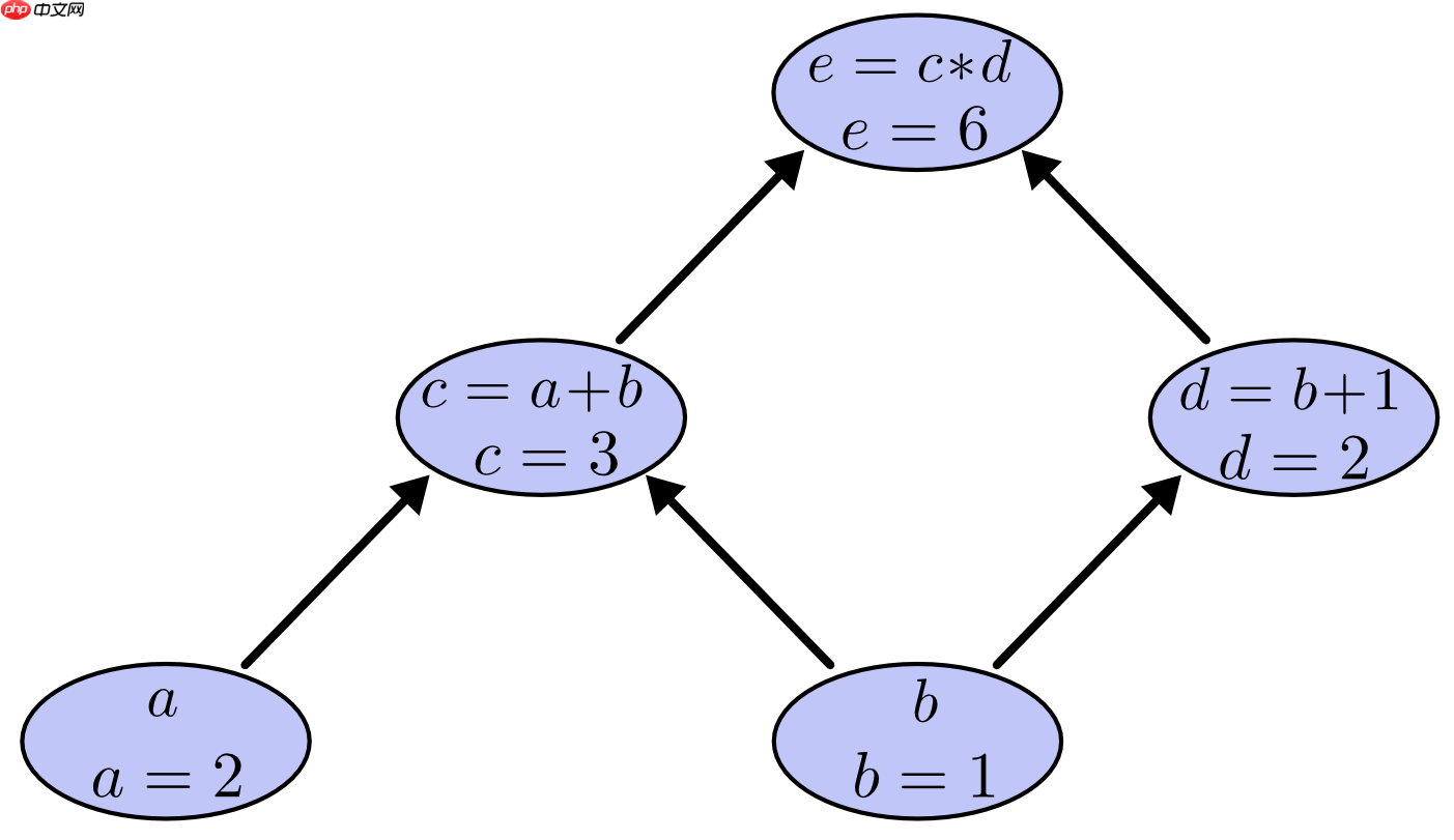
# we set requires_grad=True to let Paddle know to keep the grapha = paddle.to_tensor(2.0, stop_gradient=False)
b = paddle.to_tensor(1.0, stop_gradient=False)
c = a + b
d = b + 1e = c * dprint('c', c)print('d', d)print('e', e)

登录后复制

c Tensor(shape=[1], dtype=float32, place=CUDAPlace(0), stop_gradient=False,
       [3.])
d Tensor(shape=[1], dtype=float32, place=CUDAPlace(0), stop_gradient=False,
       [2.])
e Tensor(shape=[1], dtype=float32, place=CUDAPlace(0), stop_gradient=False,
       [6.])

登录后复制

CUDA 语义

在Paddle中我们可以很简单的在指定的GPU或者CPU上创建tensor。
在Paddle中我们可以很简单的设置数据操作的全局运行设备。

In [5]

# use cpucpu = paddle.set_device("cpu")
paddle.disable_static(cpu)
x = paddle.rand((10,))print(x)# create tensor on cpucpu_tensor = paddle.to_tensor(x, place=paddle.CPUPlace())print(cpu_tensor)

登录后复制

Tensor(shape=[10], dtype=float32, place=CPUPlace, stop_gradient=True,
       [0.53680271, 0.27223611, 0.43967441, 0.57829952, 0.21739028, 0.60926312, 0.35176951, 0.77277660, 0.14364018, 0.43463656])
Tensor(shape=[10], dtype=float32, place=CPUPlace, stop_gradient=True,
       [0.53680271, 0.27223611, 0.43967441, 0.57829952, 0.21739028, 0.60926312, 0.35176951, 0.77277660, 0.14364018, 0.43463656])

登录后复制

注：只有在Gpu环境下运行下方代码不会报错

In [6]

# use gpugpu = paddle.set_device("gpu")
paddle.disable_static(gpu)
y = x*2print(y)# create tensor on gpugpu_tensor = paddle.to_tensor(x, place=paddle.CUDAPlace(0))print(gpu_tensor)

登录后复制

Tensor(shape=[10], dtype=float32, place=CUDAPlace(0), stop_gradient=True,
       [1.07360542, 0.54447222, 0.87934881, 1.15659904, 0.43478057, 1.21852624, 0.70353901, 1.54555321, 0.28728035, 0.86927313])
Tensor(shape=[10], dtype=float32, place=CUDAPlace(0), stop_gradient=True,
       [0.53680271, 0.27223611, 0.43967441, 0.57829952, 0.21739028, 0.60926312, 0.35176951, 0.77277660, 0.14364018, 0.43463656])

登录后复制

Paddle 是一个会自动计算梯度的框架

我们知道Paddle无时无刻不在使用图，接下来我们展示一些Paddle自动计算梯度的使用案例。

函数 $f (x) = (x - 2)^{2}$ f(x)=(x−2)2.

Q: 如何计算 $\frac{d}{d x} f (x)$ dxdf(x) 以及如何计算 $f^{'} (1)$ f′(1).

我们可以先计算叶子变量(y)，然后调用backward()函数，一次性计算出y的所有所有梯度。

In [7]

def f(x):
    return (x-2)**2def fp(x):
    return 2*(x-2)

x = paddle.to_tensor([1.0], stop_gradient=False)

y = f(x)
y.backward()print('Analytical f\'(x):', fp(x))print('Paddle\'s f\'(x):', x.grad)

登录后复制

Analytical f'(x): Tensor(shape=[1], dtype=float32, place=CUDAPlace(0), stop_gradient=False,
       [-2.])
Paddle's f'(x): [-2.]

登录后复制

该方法也能计算函数的梯度。

例如 $w = [w_{1}, w_{2}]^{T}$ w=[w1,w2]T

函数 $g (w) = 2 w_{1} w_{2} + w_{2} \cos (w_{1})$ g(w)=2w1w2+w2cos(w1)

Q: 计算 $\nabla_{w} g (w)$ ∇wg(w) 并验证 $\nabla_{w} g ([π, 1]) = [2, π - 1]^{T}$ ∇wg([π,1])=[2,π−1]T

In [8]

def g(w):
    return 2*w[0]*w[1] + w[1]*paddle.fluid.layers.cos(w[0])def grad_g(w):
    return [2*w[1] - w[1]*paddle.fluid.layers.sin(w[0]), 2*w[0] + paddle.fluid.layers.cos(w[0])]

w = paddle.to_tensor([np.pi, 1], stop_gradient=False)

z = g(w)
z.backward()print('Analytical grad g(w)', grad_g(w))print('Paddle\'s grad g(w)', w.grad)

登录后复制

Analytical grad g(w) [Tensor(shape=[1], dtype=float32, place=CUDAPlace(0), stop_gradient=False,
       [2.]), Tensor(shape=[1], dtype=float32, place=CUDAPlace(0), stop_gradient=False,
       [5.28318548])]
Paddle's grad g(w) [2.        5.2831855]

登录后复制

使用梯度

我们得到梯度之后，就可以使用我们最喜欢的优化算法：梯度下降算法了！

函数 $f$ f （由上面定义并计算）.

Q: 如何计算 $x$ x 让 $f$ f最小?"

『行远见大』PaddlePaddle2.0 使用教学 - php中文网

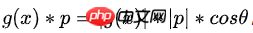
θ是两向量之间的夹角，当θ为180度得时候，g(x) * p可取到最小值，即为下降最快的方向。

所以，负梯度方向为函数f(x)下降最快的方向。如果f(x)是凸函数，则局部最优解就是全局最优解。

注：梯度下降原理可参考『行远见大』李宏毅机器学习笔记：梯度下降

线性回归

接下来，我们构造一些数据，并降低损失函数在这些数据上的计算值。

我们实现梯度下降方法来解决线性回归任务。

In [9]

import paddle.fluid as fluid
paddle.disable_static()# make a simple linear dataset with some noised = 2n = 50X = paddle.randn((n,d))
true_w = paddle.to_tensor([[-1.0], [2.0]])
y = fluid.layers.matmul(x=X, y=true_w) + paddle.randn((n,1)) * 0.1print('X shape', X.shape)print('y shape', y.shape)print('w shape', true_w.shape)

登录后复制

X shape [50, 2]
y shape [50, 1]
w shape [2, 1]

登录后复制

注意数据维度

Paddle有很多处理batch数据的操作，按照约定俗成的规则，batch数据的维度是 $(N, d)$ (N,d)，其中 $N$ N是batch的大小。

正确性检查

为了验证Paddle中梯度计算结果的正确性，我们可以调用梯度计算来计算RSS的梯度:

$\nabla_{w} L_{R S S} (w; X) = \nabla_{w} \frac{1}{n} ∣ ∣ y - X w ∣ ∣_{2}^{2} = - \frac{2}{n} X^{T} (y - X w)$ ∇wLRSS(w;X)=∇wn1∣∣y−Xw∣∣22=−n2XT(y−Xw)

Padddle梯度计算正确性验证完毕之后，接下来我们介绍如何使用梯度！

使用自动计算导数的GD来训练线性回归模型

我们接下来使用梯度来运行梯度下降算法

注意：这个例子是为了说明Paddle和我们之前所常用的一些使用方法之间的联系，在接下来的例子中，我们会看到如何使用Paddle所特有的方式来解决问题。

paddle.nn.Module

Module是Paddle处理tensor操作的一种方式。Modules是paddle.nn.Module类的子类，它的所有模块都是可调用的且能被组合成复杂函数。

paddle.nn docs

注意：Modules中大部分的功能都能通过paddle.nn.functional中的函数来访问，如何通过paddle.nn.functional中的函数来访问，需要自己创建和管理权重tensors。

paddle.nn.functional docs.

线性模型

modules的基本组成部分是带有偏置的可进行线性变换的线性模型。线性模型的输入参数为输入数据的维度和输出数据的维度，并生成线性变换权重。

AI大学堂

科大讯飞打造的AI学习平台

查看详情

和我们手动初始化 $w$ w不同的是，线性模型能自动随机初始化权重。在最小化凸损失函数过程中（比如：训练神经网络），初始化非常重要且能影响模型结果。如果训练和我们预期的不一致，手动初始化权重改变默认的初始化权重是我们的解决方案之一。Paddle在paddle.nn.initializer模块中实现了一些常见的通用初始化函数。

paddle.nn.initializer docs

In [10]

import paddleimport numpy as npimport paddle.fluid as fluidfrom paddle.fluid.dygraph import Linearfrom paddle.fluid.dygraph.base import to_variable
paddle.disable_static()

d_in = 3d_out = 4linear_module = Linear(d_in, d_out)
example_tensor = paddle.to_tensor([[1,2,3], [4,5,6]], dtype=np.float32)print('example_tensor', example_tensor.shape)# applys a linear transformation to the datatransformed = linear_module(example_tensor)print('transormed', transformed.shape)print('We can see that the weights exist in the background\n')print('W:', linear_module.weight)print('b:', linear_module.bias)

登录后复制

example_tensor [2, 3]
transormed [2, 4]
We can see that the weights exist in the background

W: Parameter containing:
Tensor(shape=[3, 4], dtype=float32, place=CUDAPlace(0), stop_gradient=False,
       [[-0.80715245,  0.15795898, -0.21465926, -0.03880989],
        [ 0.46822685,  0.65653104,  0.58932698,  0.65214843],
        [ 0.11917669, -0.26796797,  0.47791028, -0.37582973]])
b: Parameter containing:
Tensor(shape=[4], dtype=float32, place=CUDAPlace(0), stop_gradient=False,
       [0., 0., 0., 0.])

登录后复制

激活函数

Paddle实现了包括但不限于 ReLU, Tanh, and Sigmoid的一些激活函数。这些函数都是一些独立的modules，使用的时候都需要先实例化。

In [11]

import paddle# we instantiate an instance of the ReLU moduleactivation_fn = paddle.nn.ReLU() 
example_tensor = paddle.to_tensor([-1.0, 1.0, 0.0])
activated = activation_fn(example_tensor)print('example_tensor', example_tensor)print('activated', activated)

登录后复制

example_tensor Tensor(shape=[3], dtype=float32, place=CUDAPlace(0), stop_gradient=True,
       [-1.,  1.,  0.])
activated Tensor(shape=[3], dtype=float32, place=CUDAPlace(0), stop_gradient=True,
       [0., 1., 0.])

登录后复制

顺序容器

很多时候，我们需要很多Modules组合在一起计算，paddle.nn.Sequential模块给我们组合这些modules实现了一个简单易用的接口。

In [12]

import paddleimport paddle.nn as nn
paddle.disable_static()

d_in = 3d_hidden = 4d_out = 1model = nn.Sequential(
                        paddle.nn.Linear(d_in, d_hidden),
                        paddle.nn.Tanh(),
                        paddle.nn.Linear(d_hidden, d_out),
                        paddle.nn.Sigmoid()
                    )

example_tensor = paddle.to_tensor([[1.,2,3],[4,5,6]])
transformed = model(example_tensor)print('transformed', transformed.shape)

登录后复制

transformed [2, 1]

登录后复制

注意: 我们可以通过parameters()方法来访问nn.Module的所有的参数。

In [13]

params = model.parameters()for param in params:    print(param)

登录后复制

Parameter containing:
Tensor(shape=[3, 4], dtype=float32, place=CUDAPlace(0), stop_gradient=False,
       [[-0.76038808,  0.37206453,  0.86865395,  0.40551195],
        [ 0.77894390, -0.85532993,  0.24330054, -0.59385502],
        [-0.73525274,  0.85373986,  0.77308381, -0.43155381]])
Parameter containing:
Tensor(shape=[4], dtype=float32, place=CUDAPlace(0), stop_gradient=False,
       [0., 0., 0., 0.])
Parameter containing:
Tensor(shape=[4, 1], dtype=float32, place=CUDAPlace(0), stop_gradient=False,
       [[-0.74270236],
        [ 0.74238259],
        [-0.84380651],
        [-0.54089689]])
Parameter containing:
Tensor(shape=[1], dtype=float32, place=CUDAPlace(0), stop_gradient=False,
       [0.])

登录后复制

损失函数

Paddle实现了包括MSELoss 和 CrossEntropyLoss在内的很多常见的损失函数。

MSELoss

该优化器用于计算预测值和目标值的均方差误差。

paddle.nn.MSELoss(reduction='mean')

对于预测值input和目标值label：

当reduction为none时： $O u t = (i n p u t − l a b e l)^{2}$ Out=(input−label)2
当reduction为mean时： $O u t = m e a n ((i n p u t − l a b e l)^{2})$ Out=mean((input−label)2)
当reduction为sum时： $O u t = s u m ((i n p u t − l a b e l)^{2})$ Out=sum((input−label)2)

参数：

reduction (str, 可选) - 约简方式，可以是 none | mean | sum。设为 none 时不使用约简，设为 mean 时返回loss的均值，设为 sum 时返回loss的和。

MSE的一些使用注释：

input (Tensor) - 预测值，维度为 [N1,N2,...,Nk] 的多维Tensor。数据类型为float32或float64。
label (Tensor) - 目标值，维度为 [N1,N2,...,Nk] 的多维Tensor。数据类型为float32或float64。

返回：变量（Tensor）, 预测值和目标值的均方差, 数值类型与输入相同

In [14]

# MSELossimport paddleimport paddle.nn as nn
paddle.disable_static()

input_data = np.array([1.5]).astype("float32")
label_data = np.array([1.7]).astype("float32")

mse_loss = paddle.nn.MSELoss()input = paddle.to_tensor(input_data)
label = paddle.to_tensor(label_data)
output = mse_loss(input, label)print(output)

登录后复制

Tensor(shape=[1], dtype=float32, place=CUDAPlace(0), stop_gradient=True,
       [0.04000002])

登录后复制

paddle.optimizer

Paddle在paddle.optimizer模块中实现了一些基于梯度的优化函数，包括梯度下降等常见的优化方法。在最小化网络损失值的过程中，需要先获取模型参数和学习率。

优化函数不会计算梯度，我们需要调用backward()来计算梯度。我们还需要在调用backward()函数之前调用optim.clear_grad()，原因是Paddle是默认梯度累加而不是梯度更新。

paddle.optimizer docs

In [15]

import paddle
paddle.disable_static()# create a simple modelmodel = paddle.nn.Linear(1, 1)# create a simple datasetX_simple = paddle.to_tensor([[1.]])
y_simple = paddle.to_tensor([[2.]])# create our optimizeroptim = paddle.optimizer.SGD(learning_rate=1e-2, parameters=model.parameters())
mse_loss_fn = paddle.nn.loss.MSELoss()

y_hat = model(X_simple)print('model params before:', model.weight)
loss = mse_loss_fn(y_hat, y_simple)
loss.backward()
optim.clear_grad()
optim.step()print('model params after:', model.weight)

登录后复制

model params before: Parameter containing:
Tensor(shape=[1, 1], dtype=float32, place=CUDAPlace(0), stop_gradient=False,
       [[1.24595797]])
model params after: Parameter containing:
Tensor(shape=[1, 1], dtype=float32, place=CUDAPlace(0), stop_gradient=False,
       [[1.24595797]])

登录后复制

正如我们所看到的这样，参数值是朝着正确的方向在更新的。

用GD自动计算导数的线性回归和Paddle中的Modules

接下里我们结合之前所学用Paddle的方式来解决线性回归问题。

In [16]

import paddle
paddle.disable_static()

step_size = 0.1linear_module = paddle.nn.Linear(d, 1)

loss_func = paddle.nn.loss.MSELoss()

optim = paddle.optimizer.SGD(learning_rate=step_size, parameters=linear_module.parameters())print('iter,\tloss,\tw')for i in range(20):
    y_hat = linear_module(X)
    loss = loss_func(y_hat, y)
    loss.backward()
    optim.minimize(loss)
    linear_module.clear_gradients()
    optim.step()    print('{},\t{},\t{}'.format(i, loss.numpy(), linear_module.weight.reshape((1,2)).numpy()))print('\ntrue w\t\t', true_w.reshape((1, 2)).numpy())print('estimated w\t', linear_module.weight.reshape((1, 2)).numpy())

登录后复制

iter,	loss,	w
0,	[2.4269376],	[[-0.74993205  0.6965952 ]]
1,	[1.6130388],	[[-0.78610355  0.9355746 ]]
2,	[1.0776808],	[[-0.8165232  1.1301192]]
3,	[0.72409034],	[[-0.84231246  1.2886189 ]]
4,	[0.4895883],	[[-0.864328   1.4178576]]
5,	[0.33342174],	[[-0.8832312  1.5233243]]
6,	[0.22899169],	[[-0.8995388  1.6094633]]
7,	[0.15886924],	[[-0.9136598  1.6798761]]
8,	[0.11158971],	[[-0.9259224  1.7374825]]
9,	[0.07958163],	[[-0.9365936  1.7846525]]
10,	[0.05782469],	[[-0.94589347  1.82331   ]]
11,	[0.0429771],	[[-0.95400584  1.855019  ]]
12,	[0.0328052],	[[-0.96108586  1.8810512 ]]
13,	[0.02581009],	[[-0.9672658  1.9024417]]
14,	[0.02098194],	[[-0.97265935  1.9200339 ]]
15,	[0.01763758],	[[-0.977365  1.934515]]
16,	[0.01531311],	[[-0.98146844  1.9464458 ]]
17,	[0.01369224],	[[-0.9850444  1.9562843]]
18,	[0.01255846],	[[-0.9881586  1.9644045]]
19,	[0.01176308],	[[-0.9908684  1.9711125]]

true w		 [[-1.  2.]]
estimated w	 [[-0.9908684  1.9711125]]

登录后复制

Paddle中的神经网络基础

我们使用一个简单的神经网络来拟合数据。

In [17]

%matplotlib inlineimport matplotlib.pyplot as pltimport numpy as np

d = 1n = 200X = paddle.rand(shape=[n,d])
y = 4 * paddle.sin(np.pi * X) * paddle.cos(6*np.pi*X**2)

plt.scatter(X.numpy(), y.numpy())
plt.title('plot of $f(x)$')
plt.xlabel('$x$')
plt.ylabel('$y$')

plt.show()

登录后复制

/opt/conda/envs/python35-paddle120-env/lib/python3.7/site-packages/matplotlib/__init__.py:107: DeprecationWarning: Using or importing the ABCs from 'collections' instead of from 'collections.abc' is deprecated, and in 3.8 it will stop working
  from collections import MutableMapping
/opt/conda/envs/python35-paddle120-env/lib/python3.7/site-packages/matplotlib/rcsetup.py:20: DeprecationWarning: Using or importing the ABCs from 'collections' instead of from 'collections.abc' is deprecated, and in 3.8 it will stop working
  from collections import Iterable, Mapping
/opt/conda/envs/python35-paddle120-env/lib/python3.7/site-packages/matplotlib/colors.py:53: DeprecationWarning: Using or importing the ABCs from 'collections' instead of from 'collections.abc' is deprecated, and in 3.8 it will stop working
  from collections import Sized
2021-03-30 16:11:00,694 - INFO - font search path ['/opt/conda/envs/python35-paddle120-env/lib/python3.7/site-packages/matplotlib/mpl-data/fonts/ttf', '/opt/conda/envs/python35-paddle120-env/lib/python3.7/site-packages/matplotlib/mpl-data/fonts/afm', '/opt/conda/envs/python35-paddle120-env/lib/python3.7/site-packages/matplotlib/mpl-data/fonts/pdfcorefonts']
2021-03-30 16:11:01,142 - INFO - generated new fontManager
/opt/conda/envs/python35-paddle120-env/lib/python3.7/site-packages/matplotlib/cbook/__init__.py:2349: DeprecationWarning: Using or importing the ABCs from 'collections' instead of from 'collections.abc' is deprecated, and in 3.8 it will stop working
  if isinstance(obj, collections.Iterator):
/opt/conda/envs/python35-paddle120-env/lib/python3.7/site-packages/matplotlib/cbook/__init__.py:2366: DeprecationWarning: Using or importing the ABCs from 'collections' instead of from 'collections.abc' is deprecated, and in 3.8 it will stop working
  return list(data) if isinstance(data, collections.MappingView) else data

登录后复制

<Figure size 432x288 with 1 Axes>

登录后复制

我们使用了一个简单的含有两个隐藏层和Tanh激活函数的神经网络。我们可以通过调节这个神经网络的一些超参数来说明超参数是如何改变模型结果的。

In [18]

import paddle
paddle.disable_static()# feel free to play with these parametersstep_size = 0.05n_epochs = 6000n_hidden_1 = 32n_hidden_2 = 32d_out = 1neural_network = paddle.nn.Sequential(
                            paddle.nn.Linear(d, n_hidden_1), 
                            paddle.nn.Tanh(),
                            paddle.nn.Linear(n_hidden_1, n_hidden_2),
                            paddle.nn.Tanh(),
                            paddle.nn.Linear(n_hidden_2, d_out)
                            )

loss_func =  paddle.nn.loss.MSELoss()

optim = paddle.optimizer.SGD(learning_rate=step_size, parameters=neural_network.parameters())print('iter,\tloss')for i in range(n_epochs):
    y_hat = neural_network(X)
    loss = loss_func(y_hat, y)
    loss.backward()
    optim.minimize(loss)
    neural_network.clear_gradients()
    optim.step()    
    if i % (n_epochs // 10) == 0:        print('{},\t{}'.format(i, loss.numpy()))

登录后复制

iter,	loss
0,	[4.3304443]
600,	[2.4166813]
1200,	[1.8737838]
1800,	[1.2042513]
2400,	[0.8763187]
3000,	[0.37564233]
3600,	[0.10311988]
4200,	[0.08779083]
4800,	[0.07374952]
5400,	[0.06556089]

登录后复制

In [19]

X_grid = paddle.to_tensor(np.linspace(0,1,50), dtype=np.float32).reshape((-1, d))
y_hat = neural_network(X_grid)
plt.scatter(X.numpy(), y.numpy())
plt.plot(X_grid.detach().numpy(), y_hat.detach().numpy(), 'r')
plt.title('plot of $f(x)$ and $\hat{f}(x)$')
plt.xlabel('$x$')
plt.ylabel('$y$')
plt.show()

登录后复制

<>:5: DeprecationWarning: invalid escape sequence \h
<>:5: DeprecationWarning: invalid escape sequence \h
<>:5: DeprecationWarning: invalid escape sequence \h
<ipython-input-19-e3b14b1061d7>:5: DeprecationWarning: invalid escape sequence \h
  plt.title('plot of $f(x)$ and $\hat{f}(x)$')

登录后复制

<Figure size 432x288 with 1 Axes>

登录后复制

作业帮助

Momentum

除了随机梯度下降还有其他的一些优化算法：比如修改自SGD的momentum。这里我们不在详述，需要了解更多的可以点击此处学习。

在下面给出的代码中我们只修改了训练步数并且在优化函数中增加了momentum参数。注意观察momentum参数是如何在较少的迭代次数中减少训练损失的。

In [20]

# feel free to play with these parametersstep_size = 0.05momentum = 0.9n_epochs = 1500n_hidden_1 = 32n_hidden_2 = 32d_out = 1neural_network = paddle.nn.Sequential(
                            paddle.nn.Linear(d, n_hidden_1), 
                            paddle.nn.Tanh(),
                            paddle.nn.Linear(n_hidden_1, n_hidden_2),
                            paddle.nn.Tanh(),
                            paddle.nn.Linear(n_hidden_2, d_out)
                            )

loss_func = paddle.nn.MSELoss()

optim = paddle.optimizer.Momentum(learning_rate=step_size, parameters=neural_network.parameters(), momentum=momentum)print('iter,\tloss')for i in range(n_epochs):
    y_hat = neural_network(X)
    loss = loss_func(y_hat, y)
    optim.clear_grad()
    loss.backward()
    optim.step()    
    if i % (n_epochs // 10) == 0:        print('{},\t{}'.format(i, loss.numpy()))

登录后复制

iter,	loss
0,	[4.3013906]
150,	[1.9414586]
300,	[0.3890838]
450,	[0.06220616]
600,	[0.04731631]
750,	[0.03343045]
900,	[0.01029729]
1050,	[0.00483068]
1200,	[0.00385345]
1350,	[0.00348599]

登录后复制

In [21]

X_grid = paddle.to_tensor(np.linspace(0,1,50), dtype=np.float32).reshape((-1, d))
y_hat = neural_network(X_grid)
plt.scatter(X.numpy(), y.numpy())
plt.plot(X_grid.detach().numpy(), y_hat.detach().numpy(), 'r')
plt.title('plot of $f(x)$ and $\hat{f}(x)$')
plt.xlabel('$x$')
plt.ylabel('$y$')
plt.show()

登录后复制

<>:5: DeprecationWarning: invalid escape sequence \h
<>:5: DeprecationWarning: invalid escape sequence \h
<>:5: DeprecationWarning: invalid escape sequence \h
<ipython-input-21-e3b14b1061d7>:5: DeprecationWarning: invalid escape sequence \h
  plt.title('plot of $f(x)$ and $\hat{f}(x)$')

登录后复制

<Figure size 432x288 with 1 Axes>

登录后复制

交叉熵损失

到目前为止，我们在回归任务中使用了MSELoss模块。在作业中，我们需要训练一个使用交叉熵损失的分类任务。

Paddle在CrossEntropyLoss模块中实现了一个交叉熵损失版本，它的使用方法相比MSE稍有不同，因此我们在这里给出了它的一些使用注释。

input (Tensor): - 输入 Tensor ，数据类型为float32或float64。其形状为 [N,C] , 其中 C 为类别数。对于多维度的情形下，它的形状为 [N,C,d1,d2,...,dk] ，k >= 1。
label (Tensor): - 输入input对应的标签值，数据类型为int64。其形状为 [N] ，每个元素符合条件：0 <= label[i] <= C-1。对于多维度的情形下，它的形状为 [N,d1,d2,...,dk] ，k >= 1。
output (Tensor): - 计算 CrossEntropyLoss 交叉熵后的损失值。

在三个预测结果中试着输出损失函数的值。真实的标签值为 $y = [1, 1, 0]$ y=[1,1,0]。和前两个例子相对应的预测值是正确的，因为它们在正确的便签所对应的列上有更高的分数值。其中第二个例子中的预测结果具有更高的置信度和更小的损失值。最后的两个例子是分别具有更低和更高置信度的不正确的预测。

CrossEntropyLoss

paddle.nn.CrossEntropyLoss(weight=None, ignore_index=- 100, reduction='mean', soft_label=False, axis=- 1, name=None)

该优化器计算输入input和标签label间的交叉熵损失，它结合了 LogSoftmax 和 NLLLoss 的OP计算，可用于训练一个 n 类分类器。

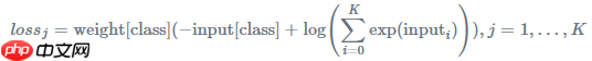
如果提供 weight 参数的话，它是一个 1-D 的tensor, 每个值对应每个类别的权重。该损失函数的数学计算公式如下：

『行远见大』PaddlePaddle2.0 使用教学 - php中文网

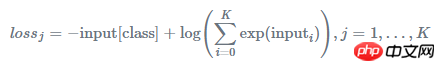
当 weight 不为 none 时，损失函数的数学计算公式为：

『行远见大』PaddlePaddle2.0 使用教学 - php中文网

参数：

weight (Tensor, 可选): - 指定每个类别的权重。其默认为 None 。如果提供该参数的话，维度必须为 C （类别数）。数据类型为float32或float64。
ignore_index (int64, 可选): - 指定一个忽略的标签值，此标签值不参与计算。默认值为-100。数据类型为int64。
reduction (str, 可选): - 指定应用于输出结果的计算方式，数据类型为string，可选值有: none, mean, sum 。默认为 mean ，计算 mini-batch loss均值。设置为 sum 时，计算 mini-batch loss的总和。设置为 none 时，则返回loss Tensor。
soft_label (bool, optional) – 指明label是否为软标签。默认为False，表示label为硬标签；若soft_label=True则表示软标签。
axis (int, optional) - 进行softmax计算的维度索引。它应该在 [−1，dim−1] 范围内，而 dim 是输入logits的维度。默认值：-1。
name (str，optional） - 操作的名称(可选，默认值为None）

In [22]

input_data = paddle.uniform([5, 100], dtype="float64")
label_data = np.random.randint(0, 100, size=(5)).astype(np.int64)
weight_data = np.random.random([100]).astype("float64")input =  paddle.to_tensor(input_data)
label =  paddle.to_tensor(label_data)
weight = paddle.to_tensor(weight_data)

ce_loss = paddle.nn.CrossEntropyLoss(weight=weight, reduction='mean')
output = ce_loss(input, label)print(output)

登录后复制

Tensor(shape=[1], dtype=float64, place=CUDAPlace(0), stop_gradient=True,
       [4.57850715])

登录后复制

学习率调度器

在训练过程中我们通常并不想使用混合学习率。Paddle提供了学习率调度器来随着训练时间的推移改变学习率。比较常用的策略是每训练一个epoch在学习率上乘以一个常数（比如0.9）或者当训练损失趋于平缓时，学习率减半。

想要获取更多的使用示例请参考学习率调度器文档。

StepDecay

StepDecay 可以让学习率按指定间隔轮数衰减。

class paddle.optimizer.lr.StepDecay(learning_rate, step_size, gamma=0.1, last_epoch=- 1, verbose=False)

learning_rate = 0.5step_size = 30gamma = 0.1learning_rate = 0.5     if epoch < 30learning_rate = 0.05    if 30 <= epoch < 60learning_rate = 0.005   if 60 <= epoch < 90

登录后复制

参数：

learning_rate (float) - 初始学习率，数据类型为Python float。
step_size (int) - 学习率衰减轮数间隔。
gamma (float, 可选) - 衰减率，new_lr = origin_lr * gamma ，衰减率必须小于等于1.0，默认值为0.1。
last_epoch (int，可选) - 上一轮的轮数，重启训练时设置为上一轮的epoch数。默认值为 -1，则为初始学习率。
verbose (bool，可选) - 如果是 True ，则在每一轮更新时在标准输出 stdout 输出一条信息。默认值为 False 。

In [23]

# train on default dynamic graph modelinear = paddle.nn.Linear(10, 10)
scheduler = paddle.optimizer.lr.StepDecay(learning_rate=0.5, step_size=5, gamma=0.8, verbose=True)
sgd = paddle.optimizer.SGD(learning_rate=scheduler, parameters=linear.parameters())for epoch in range(20):    for batch_id in range(2):
        x = paddle.uniform([10, 10])
        out = linear(x)
        loss = paddle.mean(out)
        loss.backward()
        sgd.step()
        sgd.clear_gradients()
        scheduler.step()    # If you update learning rate each step
  # scheduler.step()        # If you update learning rate each epoch# train on static graph modepaddle.enable_static()
main_prog = paddle.static.Program()
start_prog = paddle.static.Program()with paddle.static.program_guard(main_prog, start_prog):
    x = paddle.static.data(name='x', shape=[None, 4, 5])
    y = paddle.static.data(name='y', shape=[None, 4, 5])
    z = paddle.static.nn.fc(x, 100)
    loss = paddle.mean(z)
    scheduler = paddle.optimizer.lr.StepDecay(learning_rate=0.5, step_size=5, gamma=0.8, verbose=True)
    sgd = paddle.optimizer.SGD(learning_rate=scheduler)
    sgd.minimize(loss)

exe = paddle.static.Executor()
exe.run(start_prog)for epoch in range(20):    for batch_id in range(2):
        out = exe.run(
            main_prog,
            feed={                'x': np.random.randn(3, 4, 5).astype('float32'),                'y': np.random.randn(3, 4, 5).astype('float32')
            },
            fetch_list=loss.name)
        scheduler.step()    # If you update learning rate each step
  # scheduler.step()        # If you update learning rate each epoch

登录后复制

Epoch 0: StepDecay set learning rate to 0.5.
Epoch 1: StepDecay set learning rate to 0.5.
Epoch 2: StepDecay set learning rate to 0.5.
Epoch 3: StepDecay set learning rate to 0.5.
Epoch 4: StepDecay set learning rate to 0.5.
Epoch 5: StepDecay set learning rate to 0.4.
Epoch 6: StepDecay set learning rate to 0.4.
Epoch 7: StepDecay set learning rate to 0.4.
Epoch 8: StepDecay set learning rate to 0.4.
Epoch 9: StepDecay set learning rate to 0.4.
Epoch 10: StepDecay set learning rate to 0.32000000000000006.
Epoch 11: StepDecay set learning rate to 0.32000000000000006.
Epoch 12: StepDecay set learning rate to 0.32000000000000006.
Epoch 13: StepDecay set learning rate to 0.32000000000000006.
Epoch 14: StepDecay set learning rate to 0.32000000000000006.
Epoch 15: StepDecay set learning rate to 0.25600000000000006.
Epoch 16: StepDecay set learning rate to 0.25600000000000006.
Epoch 17: StepDecay set learning rate to 0.25600000000000006.
Epoch 18: StepDecay set learning rate to 0.25600000000000006.
Epoch 19: StepDecay set learning rate to 0.25600000000000006.
Epoch 20: StepDecay set learning rate to 0.20480000000000004.
Epoch 21: StepDecay set learning rate to 0.20480000000000004.
Epoch 22: StepDecay set learning rate to 0.20480000000000004.
Epoch 23: StepDecay set learning rate to 0.20480000000000004.
Epoch 24: StepDecay set learning rate to 0.20480000000000004.
Epoch 25: StepDecay set learning rate to 0.16384000000000004.
Epoch 26: StepDecay set learning rate to 0.16384000000000004.
Epoch 27: StepDecay set learning rate to 0.16384000000000004.
Epoch 28: StepDecay set learning rate to 0.16384000000000004.
Epoch 29: StepDecay set learning rate to 0.16384000000000004.
Epoch 30: StepDecay set learning rate to 0.13107200000000005.
Epoch 31: StepDecay set learning rate to 0.13107200000000005.
Epoch 32: StepDecay set learning rate to 0.13107200000000005.
Epoch 33: StepDecay set learning rate to 0.13107200000000005.
Epoch 34: StepDecay set learning rate to 0.13107200000000005.
Epoch 35: StepDecay set learning rate to 0.10485760000000004.
Epoch 36: StepDecay set learning rate to 0.10485760000000004.
Epoch 37: StepDecay set learning rate to 0.10485760000000004.
Epoch 38: StepDecay set learning rate to 0.10485760000000004.
Epoch 39: StepDecay set learning rate to 0.10485760000000004.
Epoch 40: StepDecay set learning rate to 0.08388608000000004.
Epoch 0: StepDecay set learning rate to 0.5.
Epoch 1: StepDecay set learning rate to 0.5.
Epoch 2: StepDecay set learning rate to 0.5.
Epoch 3: StepDecay set learning rate to 0.5.
Epoch 4: StepDecay set learning rate to 0.5.
Epoch 5: StepDecay set learning rate to 0.4.
Epoch 6: StepDecay set learning rate to 0.4.
Epoch 7: StepDecay set learning rate to 0.4.
Epoch 8: StepDecay set learning rate to 0.4.
Epoch 9: StepDecay set learning rate to 0.4.
Epoch 10: StepDecay set learning rate to 0.32000000000000006.
Epoch 11: StepDecay set learning rate to 0.32000000000000006.
Epoch 12: StepDecay set learning rate to 0.32000000000000006.
Epoch 13: StepDecay set learning rate to 0.32000000000000006.
Epoch 14: StepDecay set learning rate to 0.32000000000000006.
Epoch 15: StepDecay set learning rate to 0.25600000000000006.
Epoch 16: StepDecay set learning rate to 0.25600000000000006.
Epoch 17: StepDecay set learning rate to 0.25600000000000006.
Epoch 18: StepDecay set learning rate to 0.25600000000000006.
Epoch 19: StepDecay set learning rate to 0.25600000000000006.
Epoch 20: StepDecay set learning rate to 0.20480000000000004.
Epoch 21: StepDecay set learning rate to 0.20480000000000004.
Epoch 22: StepDecay set learning rate to 0.20480000000000004.
Epoch 23: StepDecay set learning rate to 0.20480000000000004.
Epoch 24: StepDecay set learning rate to 0.20480000000000004.
Epoch 25: StepDecay set learning rate to 0.16384000000000004.
Epoch 26: StepDecay set learning rate to 0.16384000000000004.
Epoch 27: StepDecay set learning rate to 0.16384000000000004.
Epoch 28: StepDecay set learning rate to 0.16384000000000004.
Epoch 29: StepDecay set learning rate to 0.16384000000000004.
Epoch 30: StepDecay set learning rate to 0.13107200000000005.
Epoch 31: StepDecay set learning rate to 0.13107200000000005.
Epoch 32: StepDecay set learning rate to 0.13107200000000005.
Epoch 33: StepDecay set learning rate to 0.13107200000000005.
Epoch 34: StepDecay set learning rate to 0.13107200000000005.
Epoch 35: StepDecay set learning rate to 0.10485760000000004.
Epoch 36: StepDecay set learning rate to 0.10485760000000004.
Epoch 37: StepDecay set learning rate to 0.10485760000000004.
Epoch 38: StepDecay set learning rate to 0.10485760000000004.
Epoch 39: StepDecay set learning rate to 0.10485760000000004.
Epoch 40: StepDecay set learning rate to 0.08388608000000004.

登录后复制

以上就是『行远见大』PaddlePaddle2.0 使用教学的详细内容，更多请关注php中文网其它相关文章！